概要
画像の画素値のヒストグラムを作成することで、画像の特性を理解し、2 値化などの処理に役立てることができます。この記事では、OpenCV の cv2.calcHist() を使用して画像のヒストグラムを作成する方法を紹介します。
画像のヒストグラム
画像のヒストグラムとは、横軸に画素値、縦軸にその画素値の頻度を取った ヒストグラム です。画像のヒストグラムを使用することで、画像の明るさやコントラストの分布を理解することができます。 カラー画像の場合、画像は複数のチャンネルで構成されているため、各チャンネルごとにヒストグラムを作成する必要があります。これにより、色ごとの画素値の分布も確認することができます。
cv2.calcHist()
OpenCV の calcHist() を使用すると、画像から指定したチャンネルのヒストグラムを計算できます。
hist = cv2.calcHist(images, channels, mask, histSize, ranges[, hist[, accumulate]])| 名前 | 型 | デフォルト値 |
|---|---|---|
| images | list of ndarray | |
| ヒストグラムを計算する画像の一覧。通常は1枚の画像をリストにして渡す。 | ||
| channels | list of int | |
| ヒストグラムを計算するチャンネルの一覧 | ||
| mask | ndarray | |
| ヒストグラムを計算する領域を指定するためのマスク画像 | ||
| histSize | list of int | |
| ヒストグラムのビンの数 | ||
| ranges | list of int | |
| ヒストグラムの範囲。この範囲外の画素値は集計対象外となる。 | ||
| 名前 | 説明 | ||
|---|---|---|---|
| hist | ヒストグラム | ||
channels、 histSize、 ranges の指定方法は少々複雑なので、詳しく見ていきます。
1 次元ヒストグラム
1 次元ヒストグラムの場合、以下のように指定します。
hist = cv2.calcHist([img], [ch], None, histSize=[bins], ranges=[l, u])chは 1 次元ヒストグラムを計算するチャンネルを指定します。binsはヒストグラムのビンの数を指定します。例えば、bins=[15]とすると、指定範囲を 15 等分します。l, uはヒストグラムを作成する範囲 $[l, u)$ を指定します。例えば、ranges=[0, 256]とすると、画素値の範囲が 0 から 255 までになります。
例えば、bins=[15], ranges=[0, 256] とした場合、$[0, 256]$ を 15 等分したビンが作成されます。

グレースケール画像のヒストグラム
グレースケール画像のヒストグラムを計算する場合、channels=[0], histSize=[ビンの数], ranges=[下限, 上限] と指定します。
import cv2
import matplotlib.pyplot as plt
import numpy as np
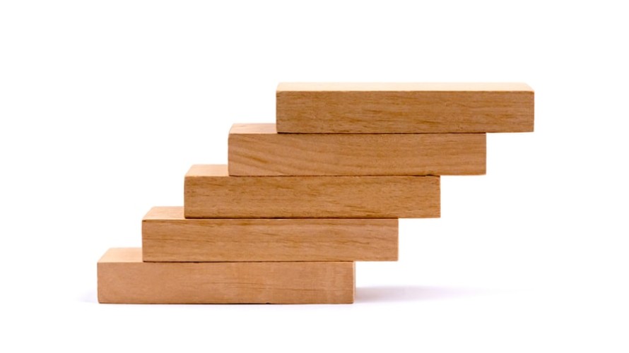
# 画像をグレースケール形式で読み込む。
img = cv2.imread("sample.jpg", cv2.IMREAD_GRAYSCALE)
# 1次元ヒストグラムを作成する。
bins_num = 100 # ビンの数
hist_range = [0, 256] # 集計範囲
hist = cv2.calcHist(
[img], channels=[0], mask=None, histSize=[bins_num], ranges=hist_range
)
hist = hist.squeeze(axis=-1) # (bins_num, 1) -> (bins_num,)matplotlib でヒストグラムを描画します。
# ヒストグラムで描画する。
def plot_hist(bins_num, hist, color):
    fig, ax = plt.subplots()

    ax.set_xticks([0, 255])
    ax.set_xlim([0, 255])
    ax.set_xlabel("Pixel Value")

    bins = np.linspace(0, 255, bins_num)
    width = bins[1] - bins[0]
    centers = bins - width
    ax.bar(centers, hist, width=width, color=color)

    plt.show()


plot_hist(bins_num, hist, color="k")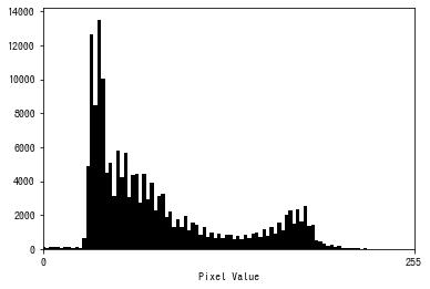
折れ線グラフで描画するコードも紹介します。
# 折れ線グラフで描画する。
def plot_hist(bins_num, hist, color):
    fig, ax = plt.subplots()

    ax.set_xticks([0, 255])
    ax.set_xlim([0, 255])
    ax.set_xlabel("Pixel Value")

    bins = np.linspace(0, 255, bins_num)
    ax.plot(bins, hist, color="k")

    plt.show()


plot_hist(bins_num, hist, color="k")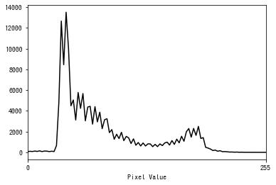
カラー画像のヒストグラム
カラー画像のヒストグラムする場合、channels=[チャンネル], histSize=[ビンの数], ranges=[下限, 上限] と指定します。
例えば、BGR 画像の場合、0 が blue、1 が green、2 が red になります。
import cv2
import matplotlib.pyplot as plt
import numpy as np


# 画像を読み込む。
img = cv2.imread("sample.jpg")

# ヒストグラムを作成する。
bins_num = 256  # ビンの数
hist_range = [0, 256]  # 集計範囲
channels = [
    {"channel": 0, "name": "blue"},
    {"channel": 1, "name": "green"},
    {"channel": 2, "name": "red"},
]

hists = []
for ch in channels:
    hist = cv2.calcHist(
        [img],
        channels=[ch["channel"]],
        mask=None,
        histSize=[bins_num],
        ranges=hist_range,
    )
    hist = hist.squeeze(axis=-1)
hists.append(hist)# 折れ線グラフで描画する。
def plot_hist(bins_num, channels, hists):
fig, ax = plt.subplots()
ax.set_xticks([0, 255])
ax.set_xlim([0, 255])
ax.set_xlabel("Pixel Value")
bins = np.linspace(0, 255, bins_num)
colors = ["b", "g", "r"]
for hist, ch in zip(hists, channels):
ax.plot(bins, hist, color=colors[ch["channel"]], label=ch["name"])
ax.legend()
plt.show()
plot_hist(bins_num, channels, hists)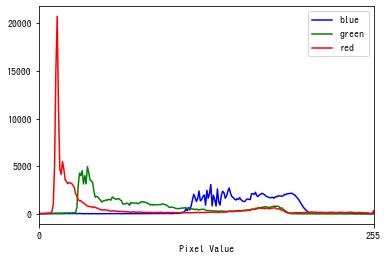
2 次元ヒストグラム
2 次元ヒストグラムの場合、以下のように指定します。
hist = cv2.calcHist(
    [img], [ch1, ch2], None, histSize=[bins1, bins2], ranges=[l1, u1, l2, u2])
ch1, ch2は 1 次元ヒストグラムを計算するチャンネルを指定します。bins1はチャンネルch1のビンの数、bins2はチャンネルch2のビンの数を指定します。l1, u1はチャンネルch1のヒストグラムを作成する範囲 $[l1, u1)$、l2, u2はチャンネルch2のヒストグラムを作成する範囲 $[l2, u2)$ を指定します。
例えば、bins=[15, 17], ranges=[0, 256, 0, 256] とした場合、$x$ 軸は [0, 256] を 15 等分、$y$ 軸は [0, 256] を 17 等分したビンが作成されます。
HSV 画像の 2 次元ヒストグラムを作成する
import itertools

import cv2
import matplotlib.pyplot as plt
import numpy as np


# 画像を読み込む。
img = cv2.imread("sample.jpg")

# HSV に変換する。
hsv = cv2.cvtColor(img, cv2.COLOR_BGR2HSV)

# 2次元ヒストグラムを作成する。
hist_range1, hist_range2 = [0, 256], [0, 256]
bins1_num, bins2_num = 20, 20
channels = [
    {"channel": 0, "name": "Hue"},
    {"channel": 1, "name": "Saturation"},
    {"channel": 2, "name": "Brightness"},
]
channel_pairs = list(itertools.combinations(channels, 2))

hists = []
for ch1, ch2 in channel_pairs:
    hist = cv2.calcHist(
        [hsv],
        channels=[ch1["channel"], ch2["channel"]],
        mask=None,
        histSize=[bins1_num, bins2_num],
        ranges=hist_range1 + hist_range2,
    )
    hists.append(hist)
2 次元ヒストグラムは、ヒストグラムの形状は 2 次元配列になるため、imshow() を使用して描画します。
def plot_hist(channel_pairs, hists):
    fig = plt.figure(figsize=(10, 10 / 3))

    for i, (hist, (ch1, ch2)) in enumerate(zip(hists, channel_pairs), 1):
        xlabel, ylabel = ch1["name"], ch2["name"]

        ax = fig.add_subplot(1, 3, i)
        fig.subplots_adjust(wspace=0.3)
        ax.imshow(hist, cmap="jet")

        # 2Dヒストグラムを描画する。
        ax.set_title(f"{xlabel} and {ylabel}")
        ax.set_xlabel(xlabel)
        ax.set_ylabel(ylabel)

    plt.show()


plot_hist(channel_pairs, hists)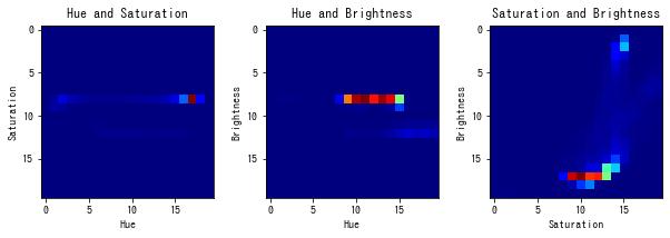
参考文献
- ディジタル画像処理 P58
- OpenCV: Histograms
コメント