
概要
OpenCV の findContours() で抽出した輪郭に対して行える処理をまとめました。
関連記事
findContours() の使い方については以下の記事を参考にしてください。
OpenCV – findContours で画像から輪郭を抽出する方法 – pystyle
輪郭抽出する
サンプルとして以下の画像を使用します。

import cv2
import numpy as np
from IPython import display
from matplotlib import pyplot as plt


def imshow(img, format=".jpg", **kwargs):
    """ndarray 配列をインラインで Notebook 上に表示する。"""
    img = cv2.imencode(format, img)[1]
    img = display.Image(img, **kwargs)
    display.display(img)


def draw_contours(img, contours, ax):
    """輪郭の点及び線を画像上に描画する。"""
    ax.imshow(img)
    ax.set_axis_off()

    for i, cnt in enumerate(contours):
        # 形状を変更する。(NumPoints, 1, 2) -> (NumPoints, 2)
        cnt = cnt.squeeze(axis=1)
        # 輪郭の点同士を結ぶ線を描画する。
        ax.add_patch(plt.Polygon(cnt, color="b", fill=None, lw=2))
        # 輪郭の点を描画する。
        ax.plot(cnt[:, 0], cnt[:, 1], "ro", mew=0, ms=4)
        # 輪郭の番号を描画する。
ax.text(cnt[0][0], cnt[0][1], i, color="r", size="20", bbox=dict(fc="w"))# 画像を読み込む。
img = cv2.imread("sample.jpg")
# グレースケールに変換する。
gray = cv2.cvtColor(img, cv2.COLOR_BGR2GRAY)
# 2値化する
ret, bin_img = cv2.threshold(gray, 20, 255, cv2.THRESH_BINARY)
# 輪郭を抽出する。
contours, hierarchy = cv2.findContours(
bin_img, cv2.RETR_EXTERNAL, cv2.CHAIN_APPROX_SIMPLE
)
fig, ax = plt.subplots(figsize=(8, 8))
draw_contours(img, contours, ax)
plt.show()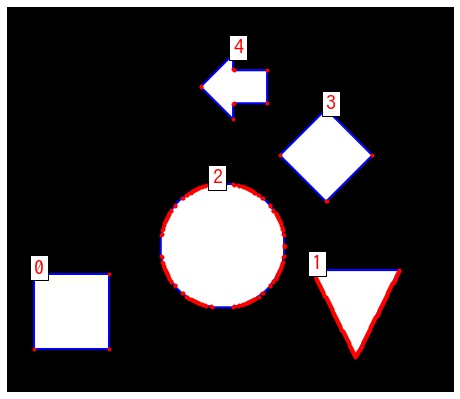
輪郭の特徴
findContours() で抽出された複数の輪郭から抽出対象の輪郭を選択するために、輪郭の点の数や面積といった情報を利用します。
| コード | |
|---|---|
| 面積 | cv2.contourArea |
| 点の数 | len |
| 輪郭の周囲の長さ | cv2.arcLength |
| 輪郭のモーメント | cv2.moments |
| 輪郭に外接する長方形 | cv2.boundingRect |
| 輪郭に外接する回転した長方形 | cv2.minAreaRect |
| 輪郭に外接する円 | cv2.minEnclosingCircle |
| 輪郭に外接する三角形 | cv2.minEnclosingTriangle |
| 輪郭に外接する楕円 | cv2.fitEllipse |
| 輪郭に対して直線フィッティング | cv2.fitLine |
| 輪郭の凸包 | cv2.convexHull |
| 輪郭が凸包かどうか | cv2.isContourConvex |
| 輪郭を少ない点で近似する | cv2.approxPolyDP |
輪郭の面積 – cv2.contourArea
cv2.contourArea() で輪郭の面積を計算できます。
retval = cv2.contourArea(contour[, oriented])- 引数
- contour: 形状が
(NumPoints, 1, 2)の numpy 配列。輪郭。 - oriented: True の場合、輪郭の点の順序が反時計回りの場合は正、時計回りの場合は負の値を返す。False の場合はいずれも正の値を返す。
- contour: 形状が
- 返り値
- points: 輪郭の面積
for i, cnt in enumerate(contours):
    # 輪郭の面積を計算する。
    area = cv2.contourArea(cnt)
    print(f"contour: {i}, area: {area}")
contour: 0, area: 4900.0 contour: 1, area: 3362.0 contour: 2, area: 10743.0 contour: 3, area: 3784.0 contour: 4, area: 1923.0
面積が閾値未満の輪郭の削除する
list(filter(lambda x: cv2.contourArea(x) > 閾値, contours)) で面積が閾値以上の輪郭のみ残せます。
contours2 = list(filter(lambda x: cv2.contourArea(x) >= 5000, contours))面積が最大の輪郭を取得する
max(contours, key=lambda x: cv2.contourArea(x)) で面積が最大の輪郭を取得できます。
max_contour = max(contours, key=lambda x: cv2.contourArea(x))輪郭の点の数
len() で輪郭を構成する点の数を取得できます。
for i, cnt in enumerate(contours):
    print(f"contour: {i}, number of points: {len(cnt)}")
contour: 0, number of points: 4 contour: 1, number of points: 165 contour: 2, number of points: 171 contour: 3, number of points: 6 contour: 4, number of points: 10
点の数で図形の種類を判定する
点の数で図形の種類を判定する場合、判定前に輪郭をより少ない数の点で構成される輪郭で近似したほうがよいでしょう。
approx_contours = []
for i, cnt in enumerate(contours):
    # 輪郭の周囲の長さを計算する。
    arclen = cv2.arcLength(cnt, True)
    # 輪郭を近似する。
    approx_cnt = cv2.approxPolyDP(cnt, epsilon=0.005 * arclen, closed=True)
approx_contours.append(approx_cnt)# 三角形を探す
triangles = list(filter(lambda x: len(x) == 3, approx_contours))
fig, ax = plt.subplots(figsize=(8, 8))
draw_contours(img, triangles, ax)
plt.show()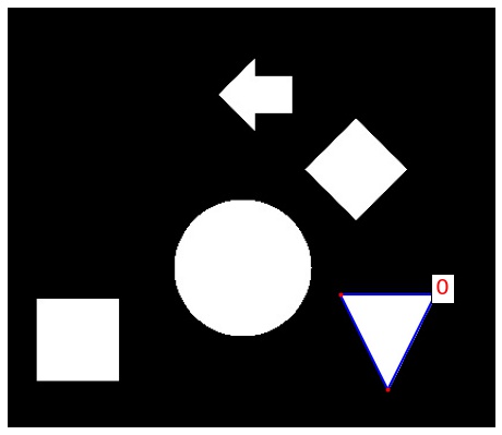
# 四角形を探す
triangles = list(filter(lambda x: len(x) == 4, approx_contours))

fig, ax = plt.subplots(figsize=(8, 8))
draw_contours(img, triangles, ax)

plt.show()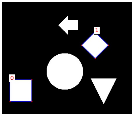
輪郭の周囲の長さ – cv2.arcLength
cv2.arcLength() で輪郭の周囲の長さを計算できます。
retval = cv2.arcLength(curve, closed)- 引数
- curve: (NumPoints, 1, 2) の numpy 配列。輪郭。
- closed: 輪郭が閉じているかどうか
- 返り値
- retval: 輪郭の長さ
for i, cnt in enumerate(contours):
    # 輪郭の周囲の長さを計算する。
    arclen = cv2.arcLength(cnt, True)
    print(f"contour: {i}, arc length: {arclen:.2f}")
contour: 0, arc length: 280.00 contour: 1, arc length: 279.97 contour: 2, arc length: 387.50 contour: 3, arc length: 245.24 contour: 4, arc length: 209.68
輪郭の重心 – cv2.moments
cv2.moments() で輪郭のモーメントを計算できます。モーメントから輪郭の重心を計算できます。
for i, cnt in enumerate(contours):
    # 輪郭のモーメントを計算する。
    M = cv2.moments(cnt)
    # モーメントから重心を計算する。
    cx = M["m10"] / M["m00"]
    cy = M["m01"] / M["m00"]
    print(f"contour: {i}, centroid: ({cx:.2f}, {cy:.2f})")
contour: 0, centroid: (60.00, 286.00) contour: 1, centroid: (327.25, 274.33) contour: 2, centroid: (202.01, 224.00) contour: 3, centroid: (299.50, 139.00) contour: 4, centroid: (215.34, 74.50)
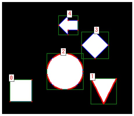
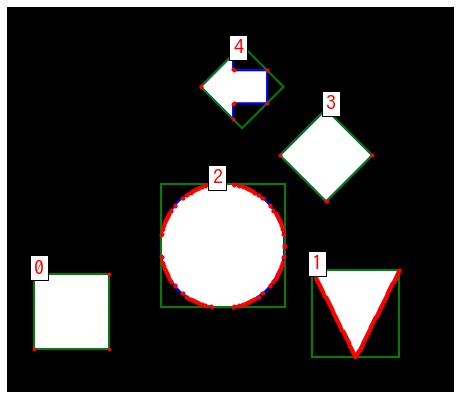
輪郭に外接する長方形 – cv2.boundingRect
cv2.boundingRect() で輪郭に外接する長方形を計算できます。
retval = cv2.boundingRect(points)- 引数
- points: (NumPoints, 1, 2) の numpy 配列。輪郭。
- 返り値
- retval: (左上の x 座標, 左上の y 座標, 幅, 高さ) であるタプル。輪郭に外接する長方形。
fig, ax = plt.subplots(figsize=(8, 8))
draw_contours(img, contours, ax)

for i, cnt in enumerate(contours):
    # 輪郭に外接する長方形を取得する。
    x, y, width, height = cv2.boundingRect(cnt)
    print(f"contour: {i}, topleft: ({x}, {y}), width: {width}, height: {height}")

    # 長方形を描画する。
    ax.add_patch(
        plt.Rectangle(xy=(x, y), width=width, height=height, color="g", fill=None, lw=2)
    )

plt.show()
contour: 0, topleft: (25, 251), width: 71, height: 71 contour: 1, topleft: (286, 247), width: 83, height: 83 contour: 2, topleft: (144, 166), width: 118, height: 117 contour: 3, topleft: (256, 96), width: 88, height: 87 contour: 4, topleft: (182, 44), width: 63, height: 62
輪郭に外接する回転した長方形 – cv2.minAreaRect
cv2.minAreaRect() で輪郭に外接する回転した長方形を計算できます。
retval = cv2.minAreaRect(points)- 引数
- points: (NumPoints, 1, 2) の numpy 配列。輪郭。
- 返り値
- retval: ((中心の x 座標, 中心の y 座標), (長方形の幅, 長方形の高さ), 回転角度) であるタプル。回転した長方形の情報。
返り値は、回転した長方形の回転中心、大きさ、回転角度です。cv2.boxPoints() により、これを長方形の 4 点の座標に変換できます。
points = cv2.boxPoints(box[, points])- 引数
- box: 回転した長方形の情報。
- points: 引数で結果を受け取る場合、指定する。
- 返り値
- points: (4, 2) の numpy 配列。回転した長方形の 4 点の座標。
fig, ax = plt.subplots(figsize=(8, 8))
draw_contours(img, contours, ax)

for i, cnt in enumerate(contours):
    # 輪郭に外接する回転した長方形を取得する。
    rect = cv2.minAreaRect(cnt)
    (cx, cy), (width, height), angle = rect
    print(
        f"contour: {i}, center: ({cx:.2f}, {cy:.2f}), "
        f"width: {width:.2f}, height: {height:.2f}, angle: {angle:.2f}"
    )

    # 回転した長方形の4点の座標を取得する。
    rect_points = cv2.boxPoints(rect)
    ax.add_patch(plt.Polygon(rect_points, color="g", fill=None, lw=2))


plt.show()
contour: 0, center: (60.00, 286.00), width: 70.00, height: 70.00, angle: -90.00 contour: 1, center: (327.00, 288.00), width: 82.00, height: 82.00, angle: -90.00 contour: 2, center: (202.50, 224.00), width: 117.00, height: 116.00, angle: -0.00 contour: 3, center: (299.50, 139.00), width: 61.52, height: 61.52, angle: -45.00 contour: 4, center: (220.50, 74.50), width: 55.15, height: 55.15, angle: -45.00
輪郭に外接する円 – cv2.minEnclosingCircle
cv2.minEnclosingCircle() で輪郭に外接する円を計算できます。
center, radius = cv2.minEnclosingCircle(points)- 引数
- points: (NumPoints, 1, 2) の numpy 配列。輪郭。
- 返り値
- center: 円の中心
- radius: 円の半径
fig, ax = plt.subplots(figsize=(8, 8))
draw_contours(img, contours, ax)

for cnt in contours:
    # 輪郭に外接する円を取得する。
    center, radius = cv2.minEnclosingCircle(cnt)
    # 描画する。
    ax.add_patch(plt.Circle(xy=center, radius=radius, color="g", fill=None, lw=2))

plt.show()
輪郭に外接する三角形 – cv2.minEnclosingTriangle
cv2.minEnclosingTriangle() で輪郭に外接する三角形を取得できます。
retval, triangle = cv2.minEnclosingTriangle(points[, triangle])- 引数
- points: (NumPoints, 1, 2) の numpy 配列。輪郭。
- triangle: 引数で結果を受け取る場合、指定する。
- 返り値
- retval: 三角形の面積
- triangle: (3, 1, 2) の numpy 配列。三角形の輪郭。
fig, ax = plt.subplots(figsize=(8, 8))
draw_contours(img, contours, ax)

for cnt in contours:
    # 輪郭に外接する三角形を取得する。
    retval, triangle = cv2.minEnclosingTriangle(cnt)
    # 描画する。
    ax.add_patch(plt.Polygon(triangle.reshape(-1, 2), color="g", fill=None, lw=2))


plt.show()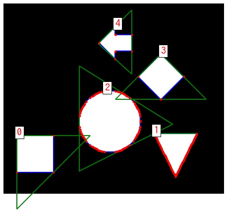
輪郭に外接する楕円 – cv2.fitEllipse
cv2.fitEllipse() で輪郭に外接する楕円を計算できます。外接する楕円の計算には、輪郭は最低 5 点以上で構成されている必要があります。
center, length, angle = cv2.fitEllipse(points)- 引数
- points: (NumPoints, 1, 2) の numpy 配列。輪郭。
- 返り値
- center: 楕円の中心
- length: 楕円の長軸、短軸の長さ
- angle: 楕円の回転角度
from matplotlib.patches import Ellipse

fig, ax = plt.subplots(figsize=(8, 8))
draw_contours(img, contours, ax)

for cnt in contours:
    # 輪郭に外接する三角形を取得する。
    if len(cnt) >= 5:
        center, (width, height), angle = cv2.fitEllipse(cnt)
        # 描画する。
        ax.add_patch(Ellipse(center, width, height, angle, color="g", fill=None, lw=2))


plt.show()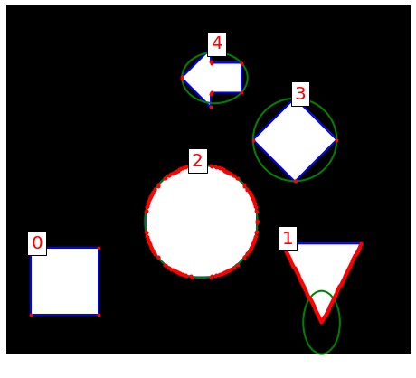
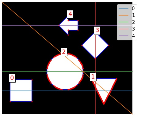
輪郭に対して直線フィッティング – cv2.fitLine
cv2.fitLine() で輪郭に対して直線フィッティングが行えます。
vx, vy, x0, y0 = cv2.fitLine(points, distType, param, reps, aeps[, line])- 引数
- points: (NumPoints, 1, 2) の numpy 配列。輪郭。
- distType: 距離関数
- param: 距離関数の係数。0 の場合、自動で決める。
- reps: 半径の解像度。
- aeps: 角度の解像度。
- 返り値
- vx、vy: vy/vx が直線の傾き
- x0, y0: 直線が通る点
返り値から直線の式は次のように求められます。
$$ f(x) = \begin{cases} \frac{vy}{vx} (x – x_0) + y_0 & vx \ne 0 \\ x_0 & vx = 0 \end{cases} $$from matplotlib.patches import Ellipse
fig, ax = plt.subplots(figsize=(8, 8))
draw_contours(img, contours, ax)
for i, cnt in enumerate(contours):
retval = cv2.fitLine(cnt, cv2.DIST_L2, 0, 0.01, 0.01)
vx, vy, x0, y0 = list(map(np.squeeze, retval))
h, w = img.shape[:2]
if vx < 0.0001:
print(f"y = {x0:.2f}")
ax.plot([x0, x0], [0, h], label=i)
else:
print(f"y = {vy:.2f}/{vx:.2f}(x - {x0:.2f}) + {y0:.2f}")
f = lambda x: vy / vx * (x - x0) + y0
ax.plot([0, w], [np.clip(f(0), 0, h), np.clip(f(w), 0, h)], label=i)
ax.legend(fontsize=15, loc="upper right")
plt.show()y = 0.00/1.00(x - 60.00) + 286.00 y = 0.71/0.71(x - 327.25) + 287.75 y = 0.00/1.00(x - 203.02) + 224.00 y = 299.50 y = 0.00/1.00(x - 212.60) + 74.50
輪郭の凸包 – cv2.convexHull
cv2.convexHull() で輪郭の凸包を計算できます。
hull = cv2.convexHull(points[, hull[, clockwise[, returnPoints]]])- 引数
- points: (NumPoints, 1, 2) の numpy 配列。輪郭
- hull: 輪郭に外接する凸包 (引数経由で受け取る場合)
- clockwise: 輪郭が時計回りかどうか
- returnPoints: 輪郭に外接する凸包を返すかどうか
- 返り値
- hull: (NumPoints, 1, 2) の numpy 配列。輪郭に外接する凸包
fig, ax = plt.subplots(figsize=(8, 8))
draw_contours(img, contours, ax)

for cnt in contours:
    # 輪郭の凸包を取得する。
    hull = cv2.convexHull(cnt)
    # 描画する。
    ax.add_patch(plt.Polygon(hull.reshape(-1, 2), color="g", fill=None, lw=2))


plt.show()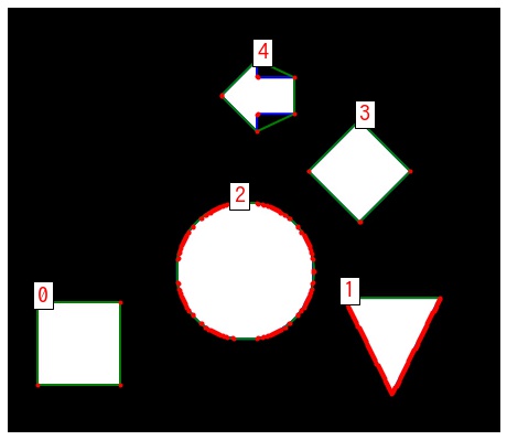
輪郭が凸包かどうか – cv2.isContourConvex
cv2.isContourConvex() で輪郭が凸包かどうかを判定できます。
retval = cv2.isContourConvex(contour)- 引数
- contour: (NumPoints, 1, 2) の numpy 配列。輪郭。
- 返り値
- retval: 輪郭が凸多角形の場合は True、そうでない場合は False を返す。
fig, ax = plt.subplots(figsize=(8, 8))
draw_contours(img, contours, ax)

for i, cnt in enumerate(contours):
    # 輪郭に外接する回転した長方形を取得する。
    is_convex = cv2.isContourConvex(cnt)
    print(f"contour: {i}, is_convex: {is_convex}")


plt.show()
contour: 0, is_convex: True contour: 1, is_convex: False contour: 2, is_convex: False contour: 3, is_convex: True contour: 4, is_convex: False
No1, 2 の図形は凸多角形であるが、結果は False となっています。 このように、輪郭検出した点は凸多角形になっていない場合があります。
輪郭を少ない点で近似する – cv2.approxPolyDP
cv2.approxPolyDP() で曲線など多数の点で構成される輪郭をより少ない点で近似できます。 処理は、Ramer-Douglas-Peucker アルゴリズム に従います。
approxCurve = cv2.approxPolyDP(curve, epsilon, closed[, approxCurve])- 引数
- curve: (NumPoints, 1, 2) の numpy 配列。輪郭
- epsilon: アルゴリズムで使用する許容距離
- closed: 輪郭が閉じているかどうか
- approxCurve: 引数で結果を受け取る場合、指定する。
- 返り値
- approxCurve: 近似した輪郭
引数の epsilon は、通常、輪郭の周囲の長さ * ratio を使用します。ratio を大きい値にするほど点の数は削減できますが、近似の精度が大雑把になります。逆に小さい値にするほど近似の精度がよくなりますが、点の数があまり削減できません。
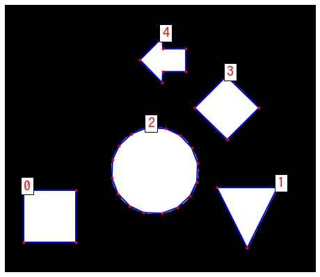
approx_contours = []
for i, cnt in enumerate(contours):
    # 輪郭の周囲の長さを計算する。
    arclen = cv2.arcLength(cnt, True)
    # 輪郭を近似する。
    approx_cnt = cv2.approxPolyDP(cnt, epsilon=0.005 * arclen, closed=True)
    approx_contours.append(approx_cnt)
    # 元の輪郭及び近似した輪郭の点の数を表示する。
    print(f"contour {i}: before: {len(cnt)}, after: {len(approx_cnt)}")

fig, ax = plt.subplots(figsize=(8, 8))
draw_contours(img, approx_contours, ax)
plt.show()
contour 0: before: 4, after: 4 contour 1: before: 165, after: 3 contour 2: before: 171, after: 16 contour 3: before: 6, after: 4 contour 4: before: 10, after: 7
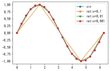
ratio による近似精度の変化
ratio を変えることで次の sin 曲線の近似がどう変化するか確認します。ratio を大きくするほど荒く近似されることがわかります。
# sin 曲線を作成する。
x = np.linspace(0, np.pi * 2, 20, dtype=np.float32)
y = np.sin(x)
contour = np.column_stack((x, y)).reshape(-1, 1, 2)

# sin 曲線を描画する。
fig, ax = plt.subplots()
ax.plot(contour[:, 0, 0], contour[:, 0, 1], "o-", label="sin")

# sin 曲線の弧長を計算する。
arclen = cv2.arcLength(contour, closed=False)

for ratio in [0.1, 0.01, 0.001]:
    # 輪郭を近似する。
    approx = cv2.approxPolyDP(contour, epsilon=ratio * arclen, closed=False)
    print(f"eps: {ratio * arclen:.2f}, number of points; {len(approx)}")
    # 近似した輪郭を描画する。
    ax.plot(approx[:, 0, 0], approx[:, 0, 1], "o-", label=f"ratio={ratio}")
ax.legend()
plt.show()
eps: 0.76, number of points; 4 eps: 0.08, number of points; 8 eps: 0.01, number of points; 18
コメント