
概要
Pytorch で使用できる最適化アルゴリズム AdaGrad、RMSProp、RMSpropGraves、Adadelta について解説します。
Adagrad
AdaGrad はこれまでのステップの勾配の大きさを記録し、学習率を調整するアルゴリズムです。
torch.optim.Adagrad(params, lr=0.01, lr_decay=0, weight_decay=0, initial_accumulator_value=0, eps=1e-10)| パラメータ | 意味 | 初期値 | 範囲 |
|---|---|---|---|
| lr | 学習率 | 0.01 | 0以上の小数 |
| lr_decay | 学習率の減衰率 | 0 | 0以上の小数 |
| weight_decay | weight decay の係数 | 0 | 0以上の小数 |
| initial_accumulator_value | 累積和の初期値 | 0 | 0以上の小数 |
| eps | epsilon | 1e-10 | 0以上の小数 |
Optimizer の状態
| パラメータ | 意味 | サイズ |
|---|---|---|
| sum | 勾配の二乗和 | パラメータ数と同じ |
学習率の減衰率が $\eta > 0$ の場合、学習率はステップごとに減衰します。
$$ \tilde{\gamma} \leftarrow \frac{\gamma}{1 + (t – 1) \eta} $$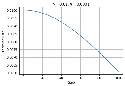
$state\_sum_t$ は勾配の二乗のステップ $t$ までの総和です。勾配の大きさを記録するのが目的のため、二乗をとっています。
$$ state\_sum_t = state\_sum_{t-1} + g^2_t = \sum_{i = 0}^t g^2_t $$$\tilde{\gamma}$ を $\sqrt{state\_sum_t}$ で割ることで学習率を調整します。序盤は $state\_sum_t$ が小さいため調整後の学習率は大きくなり、終盤は $state\_sum_t$ が大きいため調整後の学習率は小さくなります。$\epsilon$ は $state\_sum_t$ の値が小さい序盤に、除算結果が大きくなりすぎないように調整するための係数です。
$$ \theta_t \leftarrow \theta_{t – 1} – g_t \frac{\tilde{\gamma}}{\sqrt{state\_sum_t} + \epsilon} $$AdaGrad の欠点として、序盤の勾配が大きい場合に、学習が途中の段階で、調整後の学習率が小さくなってしまい、パラメータがほとんど更新されなくなることがあります。
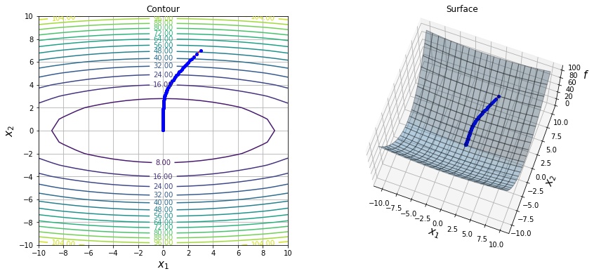
以下は $f(x, y) = 0.1 * x^2 + y^2$ という関数を lr=1.0 の AdaGrad で最適化した結果になります。

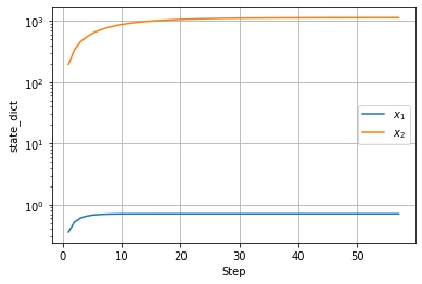
以下は $state\_dict$ の値の推移です。$x_2$ 方向は序盤の勾配が急のため、$state\_dict$ の値が急に大きくなっています。
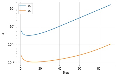
以下は調整後の学習率の値の推移です。$x_2$ 方向の $state\_dict$ に応じて学習率が調整されていることがわかります。

RMSprop、RMSpropGraves
AdaGrad では、勾配の二乗のステップ $t$ までの総和を計算し、その平方根で除算していたため、過去の勾配の大きさはすべて等しく学習率の調整に影響を与えていました。一方、RMSprop では、勾配の二乗のステップ $t$ までの指数移動平均を計算します。指数移動平均のため、直近のステップの勾配の大きさがより重視されるようになります。
torch.optim.RMSprop(params, lr=0.01, alpha=0.99, eps=1e-08, weight_decay=0, momentum=0, centered=False)| パラメータ | 意味 | 初期値 | 範囲 |
|---|---|---|---|
| lr | 学習率 | 0.01 | 0以上の小数 |
| alpha | 指数移動平均の係数 | 0.99 | 0以上の小数 |
| eps | epsilon | 1e-8 | 0以上の小数 |
| weight_decay | weight decay の係数 | 0 | 0以上の小数 |
| momentum | Momentum の係数 | 0 | 0以上の小数 |
| centered | centered RMSProp を有効にするかどうか | FALSE | bool |
Optimizer の状態
| パラメータ | 意味 | サイズ |
|---|---|---|
| momentum_buffer | Momentum のバッファ | パラメータ数と同じ |
| square_avg | 勾配の二乗の指数移動平均 | パラメータ数と同じ |
勾配の二乗の指数移動平均をとります。$\alpha$ の値が小さいほど過去の勾配の影響が弱くなります。
$$ v_t \leftarrow \alpha v_{t-1} + (1 – \alpha) g^2_t $$以下は $f(x, y) = 0.1 * x^2 + y^2$ という関数を lr=0.1, alpha=0.9 の RMSprop で最適化した結果になります。
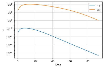
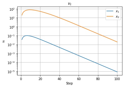
以下は $v_t$ の値の推移です。移動指数平均なので、序盤の勾配が急なところで大きくなったあと、徐々に小さくなっているのがわかります。
以下は調整後の学習率の値の推移です。$v_t$ の値に応じて学習率が調整されていることがわかります。
RMSpropGraves
centerd=True の場合、RMSpropGraves という RMSProp の改良版になります。RMSprop との違いは、勾配の二乗の指数移動平均から勾配の指数移動平均を減算するように変更されている点です。
Optimizer の状態
| パラメータ | 意味 | サイズ |
|---|---|---|
| momentum_buffer | Momentum のバッファ | パラメータ数と同じ |
| grad_avg | 勾配の指数移動平均 | パラメータ数と同じ |
| square_avg | 勾配の二乗の指数移動平均 | パラメータ数と同じ |
Adadelta
Adadelta は AdaGrad の以下の欠点を改善したアルゴリズムです。
- 学習途中で学習率が小さくなってしまう
- ベースの学習率を設定する必要がある
torch.optim.Adadelta(params, lr=1.0, rho=0.9, eps=1e-06, weight_decay=0)Adadelta の論文に記載されているアルゴリズムでは、学習率は存在しませんが、Pytorch では API の便宜上、Adadelta によって決定された学習率にスケールするためのパラメータとして lr が残っています。lr=1 とすれば、論文と同じアルゴリズムになります。
| パラメータ | 意味 | 初期値 | 範囲 |
|---|---|---|---|
| lr | 学習率 | 1.0 | 0以上の小数 |
| rho | 移動指数平均の係数 | 0.9 | 0以上の小数 |
| eps | epsilon | 1e-6 | 0以上の小数 |
| weight_decay | weight decay の係数 | 0 | 0以上の小数 |
Optimizer の状態
| パラメータ | 意味 | サイズ |
|---|---|---|
| square_avg | 勾配の二乗の指数移動平均 | パラメータ数と同じ |
| acc_delta | 更新量の移動指数平均 | パラメータ数と同じ |
学習途中で学習率が小さくなってしまう問題に関しては、RMSProp 同様、勾配の二乗和ではなく、勾配の移動指数平均を計算するように変更することで対策しました。
$$ v_t \leftarrow \rho v_{t – 1} + (1 – \rho) g^2_t $$分母の $\sqrt{u_{t – 1} + \epsilon}$ は更新量の単位をパラメータと合わせて、学習率の設定を不要にするためについています。 パラメータがそれぞれ仮想の単位を持っていると仮定したとき、パラメータの変化量はパラメータの単位に合わせて行われるべきです。 次元解析の考え方を取り入れて、SGD や AdaGrad、RMSprop の更新式を考察してみます。
SGD の次元解析
$$ \theta_t \leftarrow \theta_{t – 1} – \gamma \nabla_{\theta} f_t (\theta_{t – 1}) \\ $$$\Delta \theta_t = \theta_t – \theta_{t – 1}$ とし、$f$ の単位は無次元量であると仮定したとき、$(\text{units of } \nabla_{\theta} f (\theta)) = \frac{1}{(\text{units of } \theta)}$ であるから、
$$ (\text{units of } \Delta \theta) = \big(\text{units of } \gamma \nabla_{\theta} f (\theta) \big) = \frac{(\text{units of } \gamma)}{(\text{units of } \theta)} $$パラメータの更新量の単位 $(\text{units of } \Delta \theta)$ をパラメータの単位 $(\text{units of } \theta)$ に合わせるには、学習率の単位を
$$ (\text{units of } \gamma) = (\text{units of } \theta)^2 $$として単位を調整する必要があります。
AdaGrad、RMSprop の次元解析
$$ \begin{aligned} &g_t \leftarrow \nabla_{\theta} f_t (\theta_{t – 1}) \\ &\tilde{\gamma} \leftarrow \frac{\gamma}{1 + (t – 1) \eta} \\ &state\_sum_t \leftarrow state\_sum_{t – 1} + g^2_t \\ &\theta_t \leftarrow \theta_{t – 1} – \tilde{\gamma} \frac{g_t}{\sqrt{state\_sum_t}+\epsilon} \\ \end{aligned} $$$\Delta \theta_t = \theta_t – \theta_{t – 1}$ とし、$f, \epsilon, \eta$ の単位は無次元量であると仮定したとき、$(\text{units of } state\_sum) = \frac{1}{(\text{units of } \theta)^2}$ であるから、
$$ (\text{units of } \Delta \theta) = (\text{units of } \tilde{\gamma}) \frac{1}{(\text{units of } \theta)} (\text{units of } \theta) $$パラメータの更新量の単位 $(\text{units of } \Delta \theta)$ をパラメータの単位 $(\text{units of } \theta)$ に合わせるには、学習率の単位を
$$ (\text{units of } \gamma) = (\text{units of } \theta) $$として単位を調整する必要があります。RMSprop の $v$ も勾配の二乗の指数移動平均なので、AdaGrad と同じです。
ニュートン法の次元解析を元にした AdaDelta の単位合わせ
ニュートン法の更新量は
$$ \Delta \theta = – H^{-1} \nabla_\theta f(\theta) $$です。ただし、$H$ はヘッセ行列を表します。 次元解析を行うと、$f$ の単位は無次元量であると仮定したとき、
$$ \begin{aligned} (\text{units of } \Delta \theta) &= (\text{units of } H^{-1}) (\text{units of } \nabla_\theta f(\theta)) \\ (\text{units of } H^{-1}) &= \frac{(\text{units of } \Delta \theta)}{(\text{units of } \nabla_\theta f(\theta))} \end{aligned} $$これをニュートン法の更新量の式に代入して、
$$ (\text{units of } \Delta \theta) = \frac{(\text{units of } \Delta \theta)}{(\text{units of } \nabla_\theta f(\theta))} (\text{units of } \nabla_\theta f(\theta)) $$Adadelta では、分子に単位を揃えるために $\Delta \theta$ の二乗のステップ $t$ までの二乗の移動指数平均 $u_t$ を計算し、その値を分母に追加しています。
$$ \Delta x_t \leftarrow \frac{\sqrt{u_{t – 1} + \epsilon }}{ \sqrt{v_t + \epsilon} }g_t $$しかし、$\Delta x_t$ を計算する段階では、$u_t$ はまだわからないので、代わりに $\Delta x_t$ は滑らかに変化するという仮定をおいて、1つ前のステップの $u_{t – 1}$ で近似します。$\Delta x_t$ が計算できたら、移動指数平均 $u_t$ を更新します。
$$ u_t \leftarrow \rho u_{t – 1} + (1 – \rho) \Delta x^2_t $$AdaDelta の次元解析
$$ \begin{aligned} &g_t \leftarrow \nabla_{\theta} f_t (\theta_{t – 1}) \\ &v_t \leftarrow \rho v_{t – 1} + (1 – \rho) g^2_t \\ &\Delta x_t \leftarrow \frac{\sqrt{u_{t – 1} + \epsilon }}{ \sqrt{v_t + \epsilon} }g_t \\ &u_t \leftarrow \rho u_{t – 1} + (1 – \rho) \Delta x^2_t \\ &\theta_t \leftarrow \theta_{t – 1} – \gamma \Delta x_t \\ \end{aligned} $$$\Delta \theta_t = \theta_t – \theta_{t – 1}$ とし、$f, \epsilon, \rho, \gamma$ の単位は無次元量であると仮定したとき、
$$ \begin{aligned} (\text{units of } v) &= \frac{1}{(\text{units of } \theta)^2} \\ (\text{units of } u) &= (\text{units of } \Delta \theta)^2 \end{aligned} $$であるから、
$$ \begin{aligned} (\text{units of } \Delta \theta) &= \frac{\sqrt{(\text{units of } u)}}{ \sqrt{(\text{units of } v)} } (\text{units of } g) \\ &= (\text{units of } \Delta \theta) (\text{units of } \theta) \frac{1}{(\text{units of } \theta)} \\ &= (\text{units of } \Delta \theta) \end{aligned} $$AdaDelta の更新式は左辺と右辺の単位が一致しているため、学習率で単位を調整する必要がありません。
以下は $f(x, y) = 0.1 * x^2 + y^2$ という関数を eps=1e-3 の Adadelta で最適化した結果になります。序盤で学習率が小さくなりすぎて更新されないのを防ぐ目的でデフォルト値より大きめの値を設定しました。

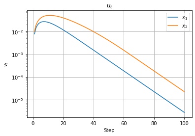
以下は $v_t, u_t$ の値の推移です。移動指数平均なので、序盤の勾配が急なところで大きくなったあと、徐々に小さくなっているのがわかります。
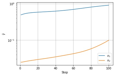
以下は調整後の学習率の値の推移です。$v_t, u_t$ の値に応じて学習率が調整されていることがわかります。
参考
- Dimensional analysis of gradient ascent — Graduate Descent: SGD の次元解析について
- 深層学習の最適化アルゴリズム – Qiita
- An overview of gradient descent optimization algorithms
- Accelerating the Adaptive Methods; RMSProp+Momentum and Adam | by Roan Gylberth | Konvergen.AI | Medium: RMSProp
- Continuing on Adaptive Method: ADADELTA and RMSProp | by Roan Gylberth | Konvergen.AI | Medium
- A short note on the AdaDelta algorithm. — Anastasios Kyrillidis
コメント