Pytorch – GAN の仕組みと Pytorch による実装例

概要

ニューラルネットワークによる生成モデル GAN (Generative Adversarial Nets) の理論的背景について解説します。

生成モデル

観測されたデータはある確率分布 $p_d$ に従う確率変数によって得られたものと仮定します。この確率分布をモデル化した $p_g$ を生成モデル (Generative Models) といいます。真の確率分布 $p_d$ に近い生成モデル $p_g$ を作成できれば、サンプリングにより、実際のデータに近いサンプルを生成することが可能となります。

例として、手書き画像データセットである MNIST について考えます。1つのサンプルは、画素数が $28 \times 28 = 784$ 、画素値が $[0, 255]$ の範囲の整数であるグレースケール画像です。 $I = \{0, 1, \cdots, 255\}$ としたとき、MNIST データセットのサンプルは $I^{784}$ の空間上に、ある確率分布 $p_d$ に従って分布していると考えます。

GAN

ニューラルネットワークを使用した生成モデルを深層生成モデル (Deep Generative Models, DGM) といいます。今回紹介する GAN (Generative Adversarial Nets) も深層生成モデルの一種です。生成モデル $p_g$ を高い表現力を持つニューラルネットワークでモデル化したことにより、画像のような高次元空間上に分布する複雑なデータを生成することが可能となりました。スタイル変換やイラストの自動着色など幅広い応用例があり、活発に研究されている分野の1つです。

GAN の構造

GANでは、Generator (生成モデル) と Discriminator (識別モデル) という2つのモデルを用意します。

Generator はノイズ $\mathbb{z}$ を入力として、偽物のデータ $\mathbb{x}$ を出力するモデルです。
Discriminator は本物または偽物のデータ $\mathbb{x}$ を入力として、そのデータが本物である確率を出力するモデルです。

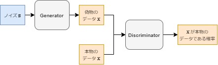
Discriminator は本物かどうかを正しく判定することを目標とする一方、Generator は Discriminator に偽物と判定されない本物に近いデータを生成することを目標として学習します。この2つのネットワークが互いに競うように、交互に学習を行うことで、本物に近いデータを生成できる Generator を作ります。

GAN の目標関数

論文では、GAN の学習を次式の最適化問題として設定しています。

\max_G \max_D V(D, G) = \max_G \max_D \mathbb{E}_{\mathbb{x} \sim p_d}\ \ [\log D(\mathbb{x})] + \mathbb{E}_{\mathbb{z} \sim p_z}\ \ [\log (1 – D(G(\mathbb{z})))]

$p_d$ : 本物のデータが従う分布
$p_z$ : ノイズが従う分布
$p_g$ : Generator が生成した偽物のデータが従う分布
$G(\mathbb{z})$ : ノイズ $\mathbb{z}$ を入力とし、データ $\mathbb{x}$ を出力する Generator
$D(\mathbb{x})$ : データ $\mathbb{x}$ を入力とし、 $\mathbb{x}$ が本物のデータである確率を出力する Discriminator

この最適化問題を解くことが、Generator 及び Discriminator の目標とどのように関係があるのかを以下で説明します。この最適化問題の理論的な解釈は以下のリンクを参照してください。

Generative Adversarial Nets: GAN の論文
An Annotated Proof of Generative Adversarial Networks with Implementation Notes: GAN 論文内の証明の詳解

Discriminator の学習

第1項 $E_{\mathbb{x} \sim p_d}\ \ [\log(D(\mathbb{x}))]$ について考えます。 $D(\mathbb{x})$ の出力は $[0, 1]$ の範囲の確率値になりますが、このとき $\log(D(\mathbb{x}))$ の値は以下のようになります。

In [1]:

import numpy as np
import matplotlib.pyplot as plt

fig, ax = plt.subplots()

x = np.linspace(0.0001, 1, 100)
y = np.log(x)

ax.plot(x, y)
ax.grid()
ax.set_xlabel("$D(\mathbb{x})$")
ax.set_ylabel("$\log(D(\mathbb{x}))$");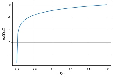

$D(\mathbb{x})$ は $p_d$ の確率分布から得られた本物のデータに対して1に近い値を出力できるようにしたいので、期待値 $E_{\mathbb{x} \sim p_d}\ \ [\log(D(\mathbb{x}))]$ が大きくなる $D$ を探します。

第2項 $\mathbb{E}_{\mathbb{z} \sim p_z}\ \ [\log (1 – D(G(\mathbb{z})))]$ について考えます。 $D(\mathbb{x})$ の出力は $[0, 1]$ の範囲の確率値になりますが、このとき $\log (1 – D(\mathbb{x})))$ の値は以下のようになります。

In [2]:

import numpy as np
import matplotlib.pyplot as plt

fig, ax = plt.subplots()

x = np.linspace(0.0001, 1, 100)
y = 1 - np.log(x)

ax.plot(x, y)
ax.grid()
ax.set_xlabel("$D(\mathbb{x})$")
ax.set_ylabel("$\log(1 - D(\mathbb{x}))$");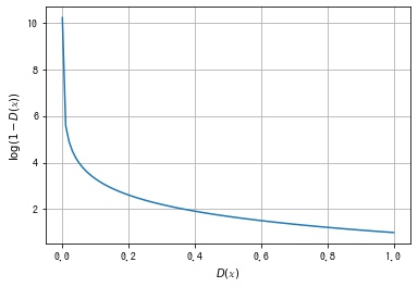

$D(\mathbb{x})$ は $p_g$ の確率分布から得られた偽物のデータに対して0に近い値を出力できるようにしたいので、期待値 $\mathbb{E}_{\mathbb{z} \sim p_z}\ \ [\log (1 – D(G(\mathbb{z})))]$ が大きくなる $D$ を探します。

したがって、入力データが本物かどうかを判別するという Discriminator の目標を達成するには、以下の最大化問題を考えればよいことがわかります。

\max_D V(D, G) = \max_D \mathbb{E}_{\mathbb{x} \sim p_d}\ \ [\log D(\mathbb{x})] + \mathbb{E}_{\mathbb{z} \sim p_z}\ \ [\log (1 – D(G(\mathbb{z})))]

この解を $D^*$ とします。

Generator の学習

Discriminator が $D^*$ に固定されたとき、次に Generator の学習について考えます。

V(D^*, G) = \mathbb{E}_{\mathbb{x} \sim p_d}\ \ [\log D^*(\mathbb{x})] + \mathbb{E}_{\mathbb{z} \sim p_z}\ \ [\log (1 – D^*(G(\mathbb{z})))]

第1項は定数なので無視し、第2項 $\mathbb{E}_{\mathbb{z} \sim p_z}\ \ [\log (1 – D^*(G(\mathbb{z})))]$ について考えます。 Generator は $p_z$ の確率分布から得られたノイズを入力として生成した偽物のデータ $G(\mathbb{z})$ に対して、Discriminator に1に近い値を出力できるようにしたいので、期待値 $\mathbb{E}_{\mathbb{z} \sim p_z}\ \ [\log (1 – D^*(G(\mathbb{z})))]$ が小さくなる $G$ を探します。

よって、以下の最小化問題を考えればよいことがわかります。

\min_G V(D, G) = \min_G \mathbb{E}_{\mathbb{x} \sim p_d}\ \ [\log D^*(\mathbb{x})] + \mathbb{E}_{\mathbb{z} \sim p_z}\ \ [\log (1 – D^*(G(\mathbb{z})))]

この解 $G^*$ が最終的に求めたい Generator です。

実装上の差異

実装上は、上記の式をそのまま実行するのではなく、以下の変更を加えます。

期待値の計算

任意のデータやノイズに関する期待値は計算できないので、標本平均に置き換えます。

$\mathbb{E}_{\mathbb{z} \sim p_z}\ \ [\log (1 – D^*(G(\mathbb{z})))]$ は、確率分布 $p_z$ からサンプリングした $n$ 個のノイズによる標本平均 $\frac{1}{n} \sum_{i = 1}^n \log (1 – D(G(\mathbb{z}_i)))$ で計算します。また、 $\mathbb{E}_{\mathbb{x} \sim p_d}\ \ [\log D^*(\mathbb{x})]$ は、学習データから $n$ 個を選択し、 $\frac{1}{n} \sum_{i = 1}^n \log D(\mathbb{x})$ で計算します。

V(D, G) = \frac{1}{n} \sum_{i = 1}^n \left( \log D(\mathbb{x}_i) + \log (1 – D(G(\mathbb{z}_i))) \right)

損失関数に binary cross entropy を使う

正解ラベルを $t_i, (i = 1, 2, \cdots, n, t_i \in \{0, 1\})$ 、出力を $y_i, (i = 1, 2, \cdots, n, y_i \in [0, 1])$ としたとき、binary cross entropy は次式になります。

BCELoss = – \sum_{i = 1}^n (t_i \log y_i + (1 – t_i) \log (1 – y_i))

Discriminator について考えます。 $\mathbb{x}_i$ が本物であるとき、出力 $D(\mathbb{x}_i)$ に対する正解ラベル $t_i$ は1なので、

\text{BCELoss}_d = – \sum_{i = 1}^n \log D(\mathbb{x}_i)

$G(\mathbb{z}_i)$ は偽物なので、出力 $D(\mathbb{x}_i)$ に対する正解ラベル $t_i$ は0なので、

\text{BCELoss}_g = – \sum_{i = 1}^n \log (1 – D(G(\mathbb{z}_i)))

よって、2つを足すと

\text{BCELoss}_d + \text{BCELoss}_g = – \sum_{i = 1}^n (\log D(\mathbb{x}_i) + \log (1 – D(\mathbb{z}_i))) = -n V(D, G)

よって、これの最小化は元の $V(D, G)$ の $D$ に関する最小化と同じことがわかります。

\underset{D}{\operatorname{minimize}} -n V(D, G) \Leftrightarrow \underset{D}{\operatorname{maximize}} V(D, G)

Generator について考えます。

$G(\mathbb{z}_i)$ を Discriminator に本物であると認識させたいので、正解ラベル $t_i$ は1となり、

\text{BCELoss} = – \sum_{i = 1}^n \log D(\mathbb{x}_i)

よって、これの最小化は元の $V(D, G)$ の $G$ に関する最小化と同じことがわかります。

\underset{G}{\operatorname{minimize}} – \sum_{i = 1}^n \log D(\mathbb{x}_i) \\ \Leftrightarrow \underset{G}{\operatorname{maximize}} – \sum_{i = 1}^n \log (1 – D(\mathbb{x}_i)) \\ \Leftrightarrow \underset{G}{\operatorname{minimize}} \sum_{i = 1}^n \log (1 – D(\mathbb{x})) \\ \Leftrightarrow \underset{G}{\operatorname{minimize}} V(D, G)

最適化の順序

論文の式だと $V(G,D)$ を $D$ について最適化してから、 $G$ について最適化しますが、実装上は、モデル $D$ を1反復分パラメータを更新し、モデル $G$ を1反復分パラメータを更新することを交互に繰り返して最適化を行います。

Pytorch の実装例

今回は MNIST データセットを利用して、手書き数字画像を生成できる Generator を作ります。モデル構造は論文では特に規定されていないので、シンプルな全結合ニューラルネットワークで作成します。

モジュールを import する

In [3]:

import matplotlib.pyplot as plt
import numpy as np
import pandas as pd
from tqdm.notebook import trange

In [4]:

import torch
import torch.nn as nn
import torch.optim as optim
import torchvision
from torchvision import datasets, transforms

デバイスを選択する

In [5]:

def get_device(gpu_id=-1):
    if gpu_id >= 0 and torch.cuda.is_available():
        return torch.device("cuda", gpu_id)
    else:
        return torch.device("cpu")


device = get_device(gpu_id=0)

Transform、Dataset、DataLoader を作成する

入力データは値の範囲を $[-1, 1]$ に正規化します。

ToTensorで PIL Image 画像を値の範囲が $[0, 1]$ のテンソルに変換します
Normalize でを値の範囲を $[-1, 1]$ に変換します

標準化とは、 $\frac{x – \text{mean}}{\text{std}}$ であるため、 $\text{mean} = 0.5, \text{std} = 0.5$ とすると、値の範囲が $[-1, 1]$ になります。

In [6]:

# Transform を作成する。
transform = transforms.Compose(
    [transforms.ToTensor(), transforms.Normalize(mean=[0.5], std=[0.5])]
)

# Dataset を作成する。
download_dir = "/data"  # ダウンロード先は適宜変更してください
dataset = datasets.MNIST(download_dir, train=True, transform=transform, download=True)

# DataLoader を作成する。
batch_size = 128  # バッチサイズ
dataloader = torch.utils.data.DataLoader(dataset, batch_size=batch_size, shuffle=True)

Generator を作成する

Generator はノイズ $\mathbb{z}$ を入力とし、データ $\mathbb{x}$ を出力するモデルになります。

In [7]:

class Generator(nn.Module):
    def __init__(self, input_dim, output_dim):
        super().__init__()
        self.main = nn.Sequential(
            # fc1
            nn.Linear(input_dim, 128),
            nn.LeakyReLU(0.2, inplace=True),
            # fc2
            nn.Linear(128, 256),
            nn.LeakyReLU(0.2, inplace=True),
            # fc3
            nn.Linear(256, 512),
            nn.LeakyReLU(0.2, inplace=True),
            # fc4
            nn.Linear(512, output_dim),
            nn.Tanh(),
        )

    def forward(self, x):
        return self.main(x)

Discriminator を作成する

Discriminator はデータ $\mathbb{x}$ を入力とし、データが本物である確率を出力するモデルになります。 $[0, 1]$ の範囲の値を出力できるように、出力層の活性化関数はシグモイド関数を使用します。

In [8]:

class Discriminator(nn.Module):
    def __init__(self, input_dim):
        super().__init__()
        self.main = nn.Sequential(
            # fc1
            nn.Linear(input_dim, 512),
            nn.LeakyReLU(0.2, inplace=True),
            nn.Dropout(0.3),
            # fc2
            nn.Linear(512, 256),
            nn.LeakyReLU(0.2, inplace=True),
            nn.Dropout(0.3),
            # fc3
            nn.Linear(256, 128),
            nn.LeakyReLU(0.2, inplace=True),
            nn.Dropout(0.3),
            # fc4
            nn.Linear(128, 1),
            nn.Sigmoid(),
            nn.Flatten(),
        )

    def forward(self, x):
        return self.main(x)

GAN を作成する

MNIST データセットの各サンプルは大きさが (28, 28) のグレースケール画像なので、データの次元数は $28 \times 28 = 784$ になります。

In [9]:

latent_dim = 100  # ノイズの次元数
data_dim = 28 * 28  # データの次元数

# 学習過程で Generator が生成する画像を可視化するためのノイズ z
fixed_z = torch.randn(100, latent_dim, device=device)

# ラベル
real_label = 1
fake_label = 0

# Generator を作成する。
G = Generator(latent_dim, data_dim).to(device)
# Discriminator を作成する。
D = Discriminator(data_dim).to(device)

損失関数とオプティマイザを作成する

損失関数は先に説明した通り、Binary Cross Entropy なので、BCELoss を使用します。

In [10]:

# 損失関数を作成する。
criterion = nn.BCELoss()

# オプティマイザを作成する。
lr = 0.0002
G_optimizer = optim.Adam(G.parameters(), lr=lr)
D_optimizer = optim.Adam(D.parameters(), lr=lr)

Discriminator を学習する関数を作成する。

In [11]:

def D_train(x):
    D.zero_grad()
    # (N, H, W) -> (N, H * W) に形状を変換する。
    x = x.flatten(start_dim=1)

    # 損失関数を計算する。
    # 本物のデータが入力の場合の Discriminator の損失関数を計算する。
    y_pred = D(x)
    y_real = torch.full_like(y_pred, real_label)
    loss_real = criterion(y_pred, y_real)

    # 偽物のデータが入力の場合の Discriminator の損失関数を計算する。
    z = torch.randn(x.size(0), latent_dim, device=device)
    y_pred = D(G(z))
    y_fake = torch.full_like(y_pred, fake_label)
    loss_fake = criterion(y_pred, y_fake)

    loss = loss_real + loss_fake

    # 逆伝搬する。
    loss.backward()

    # パラメータを更新する。
    D_optimizer.step()

    return float(loss)

Generator を学習する関数を作成する。

In [12]:

def G_train(x):
    G.zero_grad()

    # 損失関数を計算する。
    z = torch.randn(x.size(0), latent_dim, device=device)
    y_pred = D(G(z))
    y = torch.full_like(y_pred, real_label)
    loss = criterion(y_pred, y)

    # 逆伝搬する。
    loss.backward()

    # パラメータを更新する。
    G_optimizer.step()

    return float(loss)

Generator で画像を生成する関数を作成する。

データを生成するときは、勾配情報を不要なので、torch.no_grad() コンテキストで実行します。

In [13]:

def generate_img(G, fixed_z):
    with torch.no_grad():
        # 画像を生成する。
        x = G(fixed_z)

    # (N, C * H * W) -> (N, C, H, W) に形状を変換する。
    x = x.view(-1, 1, 28, 28).cpu()
    # 画像を格子状に並べる。
    img = torchvision.utils.make_grid(x, nrow=10, normalize=True, pad_value=1)
    # テンソルを PIL Image に変換する。
    img = transforms.functional.to_pil_image(img)

    return img

GAN の学習を実行する関数を作成する

In [14]:

def train_gan(n_epoch):
    G.train()
    D.train()

    history = []
    for epoch in trange(n_epoch, desc="epoch"):

        D_losses, G_losses = [], []
        for x, _ in dataloader:
            x = x.to(device)
            D_losses.append(D_train(x))
            G_losses.append(G_train(x))

        # 途中経過を確認するために画像を生成する。
        img = generate_img(G, fixed_z)

        # 途中経過を記録する。
        info = {
            "epoch": epoch + 1,
            "D_loss": np.mean(D_losses),
            "G_loss": np.mean(G_losses),
            "img": img,
        }
        history.append(info)

    history = pd.DataFrame(history)

    return history


history = train_gan(n_epoch=50)

損失関数の値の推移を描画する

In [15]:

def plot_history(history):
    fig, ax = plt.subplots()

    # 損失の推移を描画する。
    ax.set_title("Loss")
    ax.plot(history["epoch"], history["D_loss"], label="Discriminator")
    ax.plot(history["epoch"], history["G_loss"], label="Generator")
    ax.set_xlabel("Epoch")
    ax.legend()

    plt.show()


plot_history(history)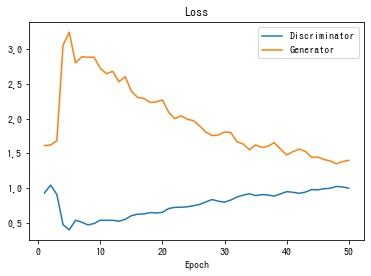

生成される画像の推移を gif 動画で保存する

pillow を使用して、各エポックの生成画像を gif 動画にして保存します。

In [16]:

def create_animation(imgs):
    """gif アニメーションにして保存する。
    """
    imgs[0].save(
        "history.gif", save_all=True, append_images=imgs[1:], duration=500, loop=0
    )


# 各エポックの画像で gif アニメーションを作成する。
create_animation(history["img"])

学習が進むにつれ、段々とはっきりした手書き数字画像が生成される様子が確認できます。

学習が終了した段階の Generator が生成する画像を表示します。

In [17]:

# 一番最後の画像を表示する。
display(history["img"].iloc[-1])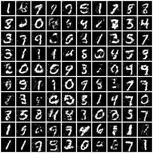

参考文献

Generative model – Wikipedia: 生成モデル
Generative Adversarial Nets: GAN の論文
An Annotated Proof of Generative Adversarial Networks with Implementation Notes: GAN 論文内の証明の詳解
GANと損失関数の計算についてまとめた – Qiita
eriklindernoren/PyTorch-GAN: PyTorch implementations of Generative Adversarial Networks.: いろいろな GAN の Pytorch での実装例
GANs from Scratch 1: A deep introduction. With code in PyTorch and TensorFlow
The GAN objective, from practice to theory and back again

コメント一覧（0件）

名無し より:

2023年1月14日 00:10

分かりやすい解説ありがとうございます。
細かい点かもしれませんが、Discriminatorの最大化問題の括弧の数が合わない気がします(Generatorも間違っているかもです)

返信
- 匿名より:
  
  2023年1月14日 01:11
  
  追記です。
  目標関数のGの箇所はminではないでしょうか
  
  返信
  - pystyle より:
    
    2023年1月14日 11:02
    
    コメント及びご指摘ありがとうございます。
    誤記があり、すみません。
    後ほど修正いたします。
    
    返信
    - pystyle より:
      
      2023年2月5日 15:21
      
      遅くなりすみません。
      ご指摘いただいた箇所を修正しました。
      ありがとうございました。
      
      返信