PRML – 「1.1 多項式曲線フィッティング」の Python 実装

概要
問題設定
訓練集合を作成する
多項式曲線フィッティング
平均平方二乗誤差 (RMSE) を確認する
係数を確認する
サンプル数を変えたときの挙動を確認する
正規化項の導入

概要

「パターン認識と機械学習上 (PRML)」の「1.1 例: 多項式曲線フィッティング」に記載されている内容を Python で再現したコードになります。書籍に記載されている説明は省略しているので、PRML と合わせて読むことが前提の記事です。

問題設定

$\sin(2 \pi x)$ の多項式曲線 (Polynomial Curve) による近似 (fitting) を考えます。

訓練集合を作成する

N: サンプル数
入力データ集合 (input data set): $\mathbf{X} = (\mathbf{x}_1, \mathbf{x}_2, \cdots, \mathbf{x}_N), \mathbf{x}_i \in \mathbb{R}^d$
目標データ集合 (target data set): $\mathbf{t} = (t_1, t_2, \cdots, t_N)^T$

今回、訓練データ集合、テストデータ集合を以下のように作成します。

訓練データ集合
- 入力データ集合は、 $[0, 1]$ から等間隔に10個選ぶ。
- 目標データ集合は、入力データ集合の各点の $\sin(2 \pi x)$ の値に正規分布に従うノイズを加えた値とする。
テストデータ集合
- 入力データ集合は、 $[0, 1]$ から等間隔に100個選ぶ。
- 目標データ集合は、入力データ集合の各点の $\sin(2 \pi x)$ の値に正規分布に従うノイズを加えた値とする。

In [1]:

import matplotlib.pyplot as plt
import numpy as np
import pandas as pd

np.random.seed(0)


def make_dataset(n, noise=False):
    x = np.linspace(0, 1, n)
    y = np.sin(2 * np.pi * x)
    if noise:
        y += np.random.normal(0, 0.2, n)

    return x, y


# 訓練集合、テスト集合を作成する。
x_train, y_train = make_dataset(10, noise=True)
x_test, y_test = make_dataset(100, noise=True)
x, y = make_dataset(100)

# 描画する。
fig, ax = plt.subplots()
ax.grid()
ax.scatter(x_train, y_train, s=50, fc="none", ec="b", label="train")
ax.plot(x, y, "g", label="$\sin(2 \pi x)$")
ax.legend()
plt.show()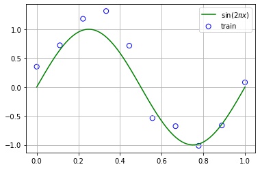

多項式曲線フィッティング

次の多項式曲線で近似します。

y(x; \mathbf{w}) = w_0 + w_1 x + w_2 x^2 + \cdots + w_M x^M = \sum_{j = 0}^M w_j x^j

$y(x; \mathbf{w})$ は係数が $\mathbf{w}$ である $x$ の関数であることを意味します。
$M$ : 多項式曲線の次数 (degree)
$\mathbf{w} = (w_0, w_1, \cdots, w_M)^T$ : 多項式曲線の係数

損失関数は二乗誤差とします。 $\frac{1}{2}$ は微分した際に式を簡潔にするためについています。

E(\mathbf{w}) = \frac{1}{2} \sum_{n = 1}^N ( y(x_n; \mathbf{w}) – t_n) )^2

この損失関数を最小化する $\mathbf{w}^*$ を求めて、 $\mathbf{w}^*$ を係数とした多項式曲線 $y(x; \mathbf{w}^*)$ で近似します。

\mathbf{w}^* = \underset{\mathbf{w}}{\text{argmin}} E(\mathbf{w})

$M = 1, 2, \cdots, 9$ のときの $y(x; \mathbf{w}^*)$ のグラフを描画してみます。

In [2]:

from sklearn.linear_model import LinearRegression


def to_polynominal_feature(degree, x):
    return np.hstack([x ** i for i in range(degree + 1)])


fig = plt.figure(figsize=(10, 10))
fig.subplots_adjust(hspace=0.4)
for i, degree in enumerate(range(10)):
    # reshape(-1, 1) で (サンプル数, 特徴量の次元数) という2次元配列にする。
    X_train = x_train.reshape(-1, 1)
    X = x.reshape(-1, 1)

    # 特徴量を生成する。[x] -> [x^0, x^1, ..., x^m]
    X_train = to_polynominal_feature(degree, X_train)
    X = to_polynominal_feature(degree, X)

    # 学習する。
    model = LinearRegression(fit_intercept=False).fit(X_train, y_train)

    # 推論する。
    y_pred = model.predict(X)

    # 描画する。
    ax = fig.add_subplot(4, 3, i + 1)
    ax.grid()
    ax.scatter(x_train, y_train, s=50, fc="none", ec="b", label="train")
    ax.plot(x, y, "g", label="$\sin(2 \pi x)$")
    ax.plot(x, y_pred, c="r", label="prediction")
    ax.set_title(f"$M$={degree}")

ax.legend(loc=(1.05, 0))
plt.show()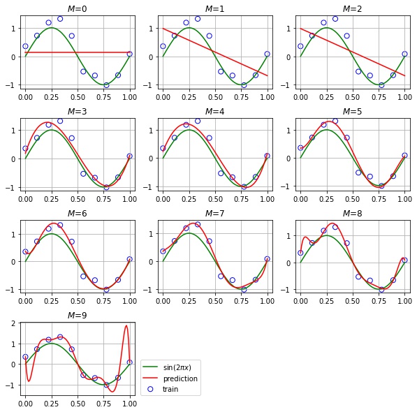

$M = 0, 1, 2$ の場合は、訓練データへの当てはまりが悪く、 $\sin(2 \pi x)$ の近似には表現力が足りていません
$M = 3, 4, 5, 6, 7$ の場合は、訓練データ、テストデータともに当てはまりがよく、 $\sin(2 \pi x)$ を上手く近似できています
$M = 8, 9$ の場合は、訓練データへの当てはまりは良いが、テストデータへの当てはまりは悪く、過学習しています

平均平方二乗誤差 (RMSE) を確認する

どのくらい近似できているかを数値的にも評価しましょう。評価には、平均平方二乗誤差 (RMSE) を使用します。

E_{RMSE} = \sqrt{\frac{2}{N} E(\mathbf{w})} = \sqrt{\frac{1}{N} \sum_{n = 1}^N ( y(x_n; \mathbf{w}) – t_n) )^2}

先程の二乗誤差と比べると、以下の利点があります。

平均をとっているため、平均平方二乗誤差の値がサンプル数 $N$ に左右されない
平方根をとっているため、目標変数 $t_n$ と単位が同じ

In [3]:

def rmse(y_true, y_pred):
    return np.sqrt(np.mean((y_true - y_pred) ** 2))


errors = []
for degree in range(10):
    # reshape(-1, 1) で (サンプル数, 特徴量の次元数) という2次元配列にする。
    X_train = x_train.reshape(-1, 1)
    X_test = x_test.reshape(-1, 1)

    # 特徴量を生成する。[x] -> [x^0, x^1, ..., x^m]
    X_train = to_polynominal_feature(degree, X_train)
    X_test = to_polynominal_feature(degree, X_test)

    # 学習する。
    model = LinearRegression(fit_intercept=False).fit(X_train, y_train)

    # 推論する。
    y_train_pred = model.predict(X_train)
    y_test_pred = model.predict(X_test)

    # RMSE を計算する。
    train_rmse = rmse(y_train, y_train_pred)
    test_rmse = rmse(y_test, y_test_pred)

    errors.append(
        {"M": degree, "train": train_rmse, "test": test_rmse, "coefficient": model.coef_,}
    )
errors = pd.DataFrame(errors)


# 描画する。
fig, ax = plt.subplots()
ax.grid()
ax.plot(errors["M"], errors["train"], "bo-", ms=10, mfc="none", label="train")
ax.plot(errors["M"], errors["test"], "ro-", ms=10, mfc="none", label="test")
ax.set_xlabel("M")
ax.set_ylabel("RMSE")
ax.legend()
plt.show()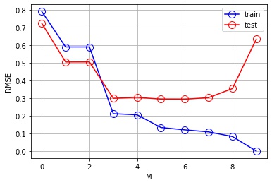

$M = 0, 1, 2$ は訓練誤差が大きく、 $\sin(2 \pi x)$ の近似には表現力が足りていません
$M = 3, 4, 5, 6, 7$ は訓練誤差、テスト誤差ともに低く、 $\sin(2 \pi x)$ を上手く近似できています
$M = 8, 9$ は訓練誤差は低いが、テスト誤差は大きくなり、過学習しています

係数を確認する

各次数における学習によって得られた係数 $\mathbf{w}^*$ の値を確認します。

In [4]:

coefs = []
index = []
for x in errors.itertuples():
    coefs.append({f"$w_{k}$": v for k, v in enumerate(x.coefficient)})
    index.append(f"$M={x.M}$")

pd.options.display.float_format = "{:.2f}".format
pd.DataFrame(coefs, index=index).fillna("")

	$w_0$	$w_1$	$w_2$	$w_3$	$w_4$	$w_5$	$w_6$	$w_7$	$w_8$	$w_9$
$M=0$	0.15
$M=1$	0.98	-1.66
$M=2$	0.97	-1.64	-0.02
$M=3$	0.18	11.39	-34.35	22.89
$M=4$	0.24	9.31	-23.83	6.01	8.44
$M=5$	0.34	-0.38	56.92	-222.22	270.05	-104.64
$M=6$	0.36	-6.09	127.41	-525.66	856.42	-626.23	173.86
$M=7$	0.36	3.13	-24.81	377.03	-1695.99	3095.93	-2527.33	771.77
$M=8$	0.35	33.28	-632.79	4962.76	-18995.39	39111.60	-44545.62	26497.25	-6431.37
$M=9$	0.35	-90.27	2220.86	-20741.11	101757.97	-289865.39	494134.29	-495988.80	270001.76	-61429.58

次数が大きいほど、係数が大きな値をとる傾向があることがわかります。

サンプル数を変えたときの挙動を確認する

次数を $M = 9$ に固定して、サンプル数を変化させたときの挙動を確認します。

In [5]:

fig = plt.figure(figsize=(7, 7))
fig.subplots_adjust(hspace=0.4)
for i, n in enumerate([10, 15, 25, 50]):
    # 訓練集合、テスト集合を作成する。
    x_train, y_train = make_dataset(n, True)
    x, y = make_dataset(100)

    # reshape(-1, 1) で (サンプル数, 特徴量の次元数) という2次元配列にする。
    X_train = x_train.reshape(-1, 1)
    X = x.reshape(-1, 1)

    # 特徴量を生成する。[x] -> [x^0, x^1, ..., x^m]
    X_train = to_polynominal_feature(9, X_train)
    X = to_polynominal_feature(9, X)

    # 学習する。
    model = LinearRegression(fit_intercept=False).fit(X_train, y_train)

    # 推論する。
    y_pred = model.predict(X)

    # 描画する。
    ax = fig.add_subplot(2, 2, i + 1)
    ax.grid()
    ax.scatter(x_train, y_train, s=30, fc="none", ec="b", label="train")
    ax.plot(x, y, "g", label="$\sin(2 \pi x)$")
    ax.plot(x, y_pred, c="r", label="prediction")
    ax.set_title(f"$N$={n}")

ax.legend(loc=(1.05, 0))
plt.show()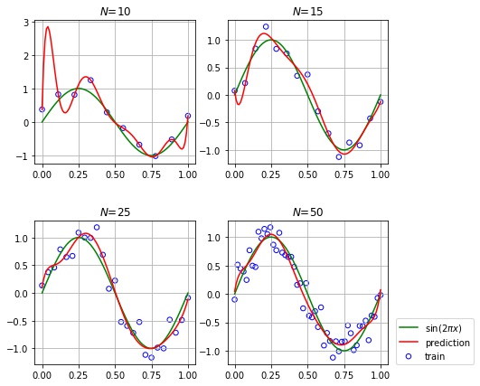

次数が多くてもサンプル数が十分大きい場合は過学習しないことがわかります。

正規化項の導入

最小化対象の二乗誤差に正規化項 $\frac{1}{2} \| \mathbf{w} \|^2$ を追加します。 $\| \mathbf{w} \|$ は係数ベクトル $\mathbf{w}$ のノルムで、各係数が大きいほど、ノルムも大きくなります。 $E(\mathbf{w})$ を最小化することは、二乗誤差を小さくしつつ、係数も小さくなるような $\mathbf{w}$ を探すことになります。

E(\mathbf{w}) = \frac{1}{2} \sum_{n = 1}^N ( y(x_n; \mathbf{w}) – t_n) )^2 + \frac{1}{2} \lambda \| \mathbf{w} \|^2

$\lambda$ は正規化項が課す制約の強さを表すパラメータです。大きいほど制約が強くなり、小さいほど制約が弱くなります。 $\lambda = 0$ とすると、正則化項がない二乗誤差になります。

$\log \lambda$ を $[-50, 0]$ の範囲で変えたときの挙動を確認します。

In [6]:

from sklearn.linear_model import Ridge

np.random.seed(0)

degree = 9

# 訓練集合、テスト集合を作成する。
x_train, y_train = make_dataset(10, noise=True)
x_test, y_test = make_dataset(100, noise=True)
x, y = make_dataset(100)

log_ls = np.linspace(-50, 0, 6)

errors = []
fig = plt.figure(figsize=(10, 6))
fig.subplots_adjust(hspace=0.4)
for i, log_l in enumerate(log_ls):
    # reshape(-1, 1) で (サンプル数, 特徴量の次元数) という2次元配列にする。
    X_train = x_train.reshape(-1, 1)
    X_test = x_test.reshape(-1, 1)
    X = x.reshape(-1, 1)

    # 特徴量を生成する。[x] -> [x^0, x^1, ..., x^m]
    X_train = to_polynominal_feature(degree, X_train)
    X_test = to_polynominal_feature(degree, X_test)
    X = to_polynominal_feature(degree, X)

    # 学習する。
    model = Ridge(alpha=np.exp(log_l), fit_intercept=False).fit(X_train, y_train)

    # 推論する。
    y_train_pred = model.predict(X_train)
    y_test_pred = model.predict(X_test)
    y_pred = model.predict(X)

    # RMSE を計算する。
    train_rmse = rmse(y_train, y_train_pred)
    test_rmse = rmse(y_test, y_test_pred)

    # 描画する。
    ax = fig.add_subplot(2, 3, i + 1)
    ax.grid()
    ax.scatter(x_train, y_train, s=50, fc="none", ec="b", label="train")
    ax.plot(x, y, "g", label="$\sin(2 \pi x)$")
    ax.plot(x, y_pred, c="r", label="prediction")
    ax.set_title(f"$\log \lambda$={log_l}")

    errors.append(
        {
            "log_lambda": log_l,
            "train": train_rmse,
            "test": test_rmse,
            "coefficient": model.coef_,
        }
    )
errors = pd.DataFrame(errors)

ax.legend(loc=(1.05, 0))
plt.show()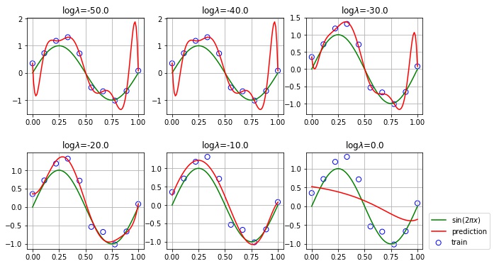

$\log \lambda = -50, -40, -30$ では、制約が弱すぎるため、過学習の傾向が見られます。
$\log \lambda = -20, -10$ ではそれなりに近似できています。
$\log \lambda = 0$ では、制約が強すぎるため、 $\sin(2 \pi x)$ を表現できなくなっています。

In [7]:

coefs = []
index = []
for x in errors.itertuples():
    coefs.append({f"$w_{k}$": v for k, v in enumerate(x.coefficient)})
    index.append(fr"$\log \lambda={x.log_lambda}$")
pd.options.display.float_format = "{:.2f}".format
pd.DataFrame(coefs, index=index).fillna("")

	$w_0$	$w_1$	$w_2$	$w_3$	$w_4$	$w_5$	$w_6$	$w_7$	$w_8$	$w_9$
$\log \lambda=-50.0$	0.35	-90.49	2226.13	-20788.42	101979.48	-290466.89	495116.24	-496938.63	270503.06	-61540.74
$\log \lambda=-40.0$	0.35	-90.49	2226.13	-20788.42	101979.48	-290466.89	495116.24	-496938.63	270503.06	-61540.74
$\log \lambda=-30.0$	0.35	-30.28	839.32	-8336.90	43671.44	-132098.74	236528.98	-246766.87	138448.10	-32255.31
$\log \lambda=-20.0$	0.36	-0.75	41.34	-40.01	-385.48	802.71	-197.68	-606.72	460.80	-74.48
$\log \lambda=-10.0$	0.27	6.93	-8.90	-16.09	2.98	12.66	10.40	2.98	-3.87	-7.29
$\log \lambda=0.0$	0.52	-0.41	-0.47	-0.33	-0.18	-0.05	0.05	0.12	0.18	0.23

制約を強くするほど、係数が小さくなっていることが確認できました。 $\log \lambda$ を変化させたときの平均平方二乗誤差の値も確認します。

In [8]:

# 描画する。
fig, ax = plt.subplots()
ax.grid()
ax.plot(errors["log_lambda"], errors["train"], "bo-", ms=10, mfc="none", label="train")
ax.plot(errors["log_lambda"], errors["test"], "ro-", ms=10, mfc="none", label="test")
ax.set_xlabel("$\log \lambda$")
ax.set_ylabel("RMSE")
ax.legend()
plt.show()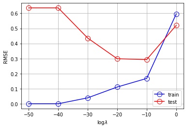

$\log \lambda = -50, -40, -30$ では、訓練誤差は低いが、テスト誤差は大きくなり、過学習しています
$\log \lambda = -20, -10$ ではそれなりに近似できています
$\log \lambda = 0$ では、訓練誤差が大きく、 $\sin(2 \pi x)$ の近似には表現力が足りていません

PRML – 「1.1 多項式曲線フィッティング」の Python 実装

概要

問題設定

訓練集合を作成する

多項式曲線フィッティング

平均平方二乗誤差 (RMSE) を確認する

係数を確認する

サンプル数を変えたときの挙動を確認する

正規化項の導入

コメント

コメントするコメントをキャンセル

PRML – 「1.1 多項式曲線フィッティング」の Python 実装

概要

問題設定

訓練集合を作成する

多項式曲線フィッティング

平均平方二乗誤差 (RMSE) を確認する

係数を確認する

サンプル数を変えたときの挙動を確認する

正規化項の導入

コメント

コメントする コメントをキャンセル

コメントするコメントをキャンセル