
概要
正規分布の最尤推定量のバイアスについて考察し、Python で検証します。
定義 – 不偏推定量
$\Theta$ をパラメータ空間としたとき、任意の $\theta \in \Theta$ に対して、
$$ E_\theta[T(X)] = \theta $$となる推定量 $T(X)$ を不偏推定量 (unbiased estimator) といいます。つまり、不偏推定量の期待値は、パラメータの値に等しいことを意味します。
正規分布の最尤推定におけるバイアス
$X = (X_1, X_2, \cdots, X_N)$ を母集団分布が平均 $\mu$、分散 $\sigma^2$ に従う正規分布のランダム標本とし、平均及び分散の最尤推定量をそれぞれ $\hat{\theta}(X) = \frac{1}{N} \sum_{i = 1}^N X_i, \hat{\sigma}^2(X) = \frac{1}{N} \sum_{i = 1}^N (X_i – \hat{\theta}(X))^2$ とします。
平均の最尤推定量の期待値は、
$$ \begin{aligned} E[\hat{\mu}(X)] &= E \left[ \frac{1}{N} \sum_{i = 1}^N X_i \right] \\ &= \frac{1}{N} \sum_{i = 1}^N E[X_i] \\ &= \frac{1}{N} N E[X_i] \\ &= \mu \end{aligned} $$よって、平均の最尤推定量 $\hat{\theta}(X)$ の期待値は、真のパラメータ $\mu$ に一致するので、不偏推定量であることがわかります。
分散の最尤推定量の期待値は、
$$ \begin{aligned} E[\hat{\sigma}^2(X)] &= E \left[ \frac{1}{N} \sum_{i = 1}^N (X_i – \hat{\mu}(X))^2 \right] \\ &= \frac{1}{N} E\left[ \sum_{i = 1}^N X_i^2 – 2 \sum_{i = 1}^N X_i \hat{\mu}(X) + \sum_{i = 1}^N \hat{\mu}(X)^2 \right] \\ &= \frac{1}{N} E\left[ \sum_{i = 1}^N X_i^2 – 2 N \hat{\mu}(X)^2 + N \hat{\mu}(X)^2 \right] \\ &= \frac{1}{N} \sum_{i = 1}^N E[X_i^2] – E[\hat{\mu}(X)^2] \\ &= E[X^2] – E[\hat{\mu}(X)^2] \end{aligned} $$$V[X] = E[X^2] – (E[X])^2$ より、
$$ \begin{aligned} E[X^2] – E[\hat{\mu}(X)^2] &= V[X] + (E[X])^2 – V[\hat{\mu}(X)] – (E[\hat{\mu}(X)])^2 \\ &= \sigma^2 + \mu^2 – V[\hat{\mu}(X)] – \mu^2 \end{aligned} $$ここで、
$$ V[\hat{\mu}(X)] = V \left[\frac{1}{N} \sum_{i = 1}^N X_i \right] = \frac{1}{N^2} \sum_{i = 1}^N V[X_i] = \frac{1}{N} \sigma^2 $$したがって、
$$ \begin{aligned} E[\hat{\sigma}^2(X)] &= \sigma^2 + \mu^2 – \frac{1}{N} \sigma^2 – \mu^2 \\ &= \frac{N – 1}{N} \sigma^2 \end{aligned} $$分散の最尤推定量 $\hat{\sigma}^2(X)$ の期待値は、真のパラメータ $\sigma^2$ に一致しないので、不偏推定量でないことがわかります。
Maximum Likelihood Estimator for Variance is Biased: Proof
Python で確認する
母集団分布が $\mu = 0, \sigma = 2$ の正規分布であるサイズ $N= 20$ のランダム標本を使って、最尤推定を行い、以下の3つのグラフを描画します。
- $\mu = 0, \sigma = 2$ の正規分布の確率密度関数 (緑)
- $\mu = E[\hat{\mu}(X)], \sigma = E[\hat{\sigma}^2(X)]$ の正規分布の確率密度関数 (赤)
- バイアスを補正した $\mu = E[\hat{\mu}(X)], \sigma = \frac{N}{N – 1} E[\hat{\sigma}^2(X)]$ の正規分布の確率密度関数 (青)
- 最尤推定量の期待値は $M = 1000$ 回の平均で計算します。
import matplotlib.pyplot as plt
import numpy as np
from scipy.stats import norm

np.random.seed(0)

mu = 0  # 平均
sigma = 2  # 標準偏差
M = 1000  # 試行回数
N = 20  # サンプル数


def mle(N):
    # 平均及び標準偏差の最尤推定量の平均をとる
    preds = []
    for i in range(M):
        X = norm.rvs(mu, sigma, size=N)
        preds.append(norm.fit(X))

    return np.mean(preds, axis=0)


fig, ax = plt.subplots()
mu_pred, sigma_pred = mle(N)

# μ=mu, σ=sigma の正規分布の確率密度関数を描画する
xs = np.linspace(-3, 3, 100)
ys = norm.pdf(xs, loc=mu, scale=sigma)
ax.plot(xs, ys, "g", label=f"true")

# μ=mu_pred, σ=sigma_pred の正規分布の確率密度関数を描画する
ys = norm.pdf(xs, loc=mu_pred, scale=sigma_pred)
ax.plot(xs, ys, "r", label=f"estimate")

# sigma_pred からバイアスを除いた正規分布の確率密度関数を描画する
unbiased = sigma_pred * N / (N - 1)
ys = norm.pdf(xs, loc=mu_pred, scale=unbiased)
ax.plot(xs, ys, "b", label=f"estimate (unbiased)")
print(f"mu={mu_pred:.2f}, sigma={sigma_pred:.2f}, sigma (unbiased)={unbiased:.2f}")

ax.grid()
ax.legend(loc=(1.05, 0))

plt.show()
mu=-0.01, sigma=1.91, sigma (unbiased)=2.01
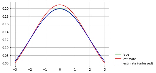
バイアスがあるため、標準偏差の最尤推定量の期待値は真の標準偏差とずれていますが、$\frac{N}{N- 1}$ 倍にスケールすることで、バイアスを除けることが確認できました。
コメント