matplotlib – hist でヒストグラムを作成する方法

概要

matplotlib でヒストグラムを作成する方法について解説します。

pyplot.hist

matplotlib.pyplot.hist(x, bins=None, range=None, density=False, weights=None, cumulative=False, bottom=None, histtype="bar", align="mid", orientation="vertical", rwidth=None, log=False, color=None, label=None, stacked=False, *, data=None, **kwargs)

引数

名前	型	デフォルト値
x	(n,) array or sequence of (n,) arrays
x	入力値は、単一の配列または配列のシーケンス (各配列は同じ長さでなくてよい) のいずれかを取ります。
bins	int or sequence or str	None, (rcParams[“hist.bins”] (デフォルト: 10))
bins	bins が整数の場合、範囲内に等幅のビンを定義します。 bins がシーケンスの場合、最初のビンの左端と最後のビンの右端を含むビンの端を定義します。この場合、ビンの間隔は不均等になることがあります。最後の（右端の）ビン以外はすべて半開区間です。言い換えれば、ビンが [1, 2, 3, 4] とすると、最初のビンは [1, 2) (1を含むが2を含まない)、2番目のビンは [2, 3] となります。しかし、最後のビンは4を含む[3, 4] となります。 bins が文字列の場合は、numpy.histogram_bin_edges() がサポートする binning 引数と解釈されます。[“auto”, “fd”, “doane”, “scott”, “stone”, “rice”, “sturges”, “sqrt”] のいずれか。
range	tuple or None, default: None	None
range	最初のビンの左端と最後のビンの右端を指定します。この範囲外の値は集計の際に無視されます。省略した場合は (x.min(), x.max()) となります。bins がシーケンスの場合は、この引数は無視されます。
density	bool, default: False	False
density	True の場合、確率密度になるように正規化します。各ビンは、ビンの度数をデータ総数とビンの幅で割ったもの (density = counts / (sum(counts) np.diff(bins)))* を表示し、ヒストグラムの下側の面積が 1 になります (np.sum(density np.diff(bins)) == 1)*。
weights	(n,) array-like or None, default: None	None
weights	x と同じ形状の配列。x にこの値を乗算した数を元にヒストグラムを作成します。
cumulative	bool or -1, default: False	False
cumulative	True の場合、ヒストグラムが計算され、各ビンにはそのビンの度数と、より小さな値のすべてのビンの度数を累積した値が表示されます。最後のビンは、データポイントの総数を表します。
bottom	array-like, scalar, or None, default: None	None
bottom	各棒の下端の位置。スカラーの場合，各棒の底は同じ量だけシフトされます。配列の場合は、各棒が独立してシフトされ、bottom の長さはビンの数と一致しなければなりません。None の場合、デフォルトは 0 です。
histtype	{“bar”, “barstacked”, “step”, “stepfilled”}	“bar”
histtype	描画するヒストグラムの種類。
align	{“left”, “mid”, “right”}	“mid”
align	棒の水平方向の配置。
orientation	{“vertical”, “horizontal”}	“vertical”
orientation	“horizontal” の場合、bottom は棒の左端と解釈されます。
rwidth	float or None, default: None	None
rwidth	棒の幅をビンの幅の何分の一かで相対的に定義します。Noneの場合は、自動的に幅を計算します。
log	bool, default: False	False
log	True の場合、ヒストグラムの軸はログスケールに設定されます。log が True で x が1次元配列の場合、空のビンは除かれ、空でないもののみが返されます。
color	color or array-like of colors or None, default: None	None
color	色または色のシーケンス。デフォルトは、折れ線を描画する場合のシーケンスと同じ色を使用します。
label	str or None, default: None	None
label	複数のデータに対応する文字列。棒グラフはデータセットごとに複数のパッチを生成しますが、最初のパッチだけがラベルを取得するので、凡例は期待通りに動作します。
stacked	bool, default: False	False
stacked	True の場合は、複数のデータを重ねて配置します。False の場合は、histtype が “bar” の場合は複数のデータを並べて配置し、histtype が “step” の場合は重ねて配置します。

返り値

名前	説明
array or list of arrays	ヒストグラムのビンの値。入力 x が配列の場合、これは長さ nbins の配列です。入力が配列 [data1, data2, …] のシーケンスの場合、これは配列のリストであり、各配列のヒストグラムの値が同じ順番で表されます。配列 n（またはその要素配列）の dtype は，重み付けや正規化が行われていなくても、常に float となります。
array	ビンの端。最初のビンの左端と最後のビンの右端を含む長さ nbins + 1 の配列。複数のデータセットが渡された場合でも、常に単一の配列。
BarContainer or list of a single Polygon or list of such objects	複数の入力データセットがある場合、ヒストグラムまたはそのようなコンテナのリストを作成するために使用される個々の Artist のコンテナ。

データの指定方法

単一の配列を渡した場合、そのヒストグラムを作成します。

In [1]:

import numpy as np
from matplotlib import pyplot as plt

np.random.seed(0)

x = np.random.normal(65, 15, 200).clip(0, 100)

fig, ax = plt.subplots()
ax.hist(x, ec="k")

plt.show()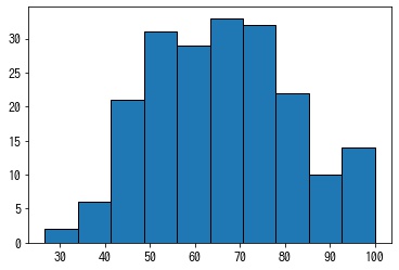

配列のシーケンスを渡した場合、各配列ごとにヒストグラムを作成し、色分けして表示します。 labels 引数で凡例に使用するラベルを指定できます。

In [2]:

np.random.seed(0)

x1 = np.random.normal(65, 15, 200).clip(0, 100)
x2 = np.random.normal(65, 15, 150).clip(0, 100)
x3 = np.random.normal(65, 15, 250).clip(0, 100)
X = [x1, x2, x3]

fig, ax = plt.subplots()
ax.hist(X, label=["x1", "x2", "x3"], ec="k")
ax.legend()

plt.show()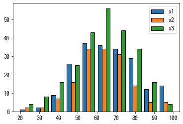

ビンの指定方法

bins に整数を指定した場合、range の範囲を bins 等分してビンを作成します。

In [3]:

np.random.seed(0)

x = np.random.normal(65, 15, 200).clip(0, 100)

fig, ax = plt.subplots()
ax.hist(x, bins=20, ec="k")

plt.show()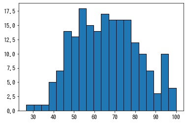

bins がシーケンスの場合、各ビンの端と解釈されます。

In [4]:

np.random.seed(0)

x = np.random.normal(65, 15, 200).clip(0, 100)

bins = np.linspace(0, 100, 11)
print(bins)

fig, ax = plt.subplots()
ax.hist(x, bins=bins, ec="k")

plt.show()

[  0.  10.  20.  30.  40.  50.  60.  70.  80.  90. 100.]

ヒストグラムを正規化する

density=True の場合、確率密度関数になるように正規化します。つまり、各ビンの幅にそのビンの度数を乗算した総和が1になります。ビンの度数の総和が1になるように正規化されるわけではないことに注意してください。

In [5]:

np.random.seed(0)

x = np.random.normal(65, 15, 200).clip(0, 100)

fig, ax = plt.subplots()
n, bins, patches = ax.hist(x, density=True, ec="k")

plt.show()

# 総和が1
print((np.diff(bins) * n).sum())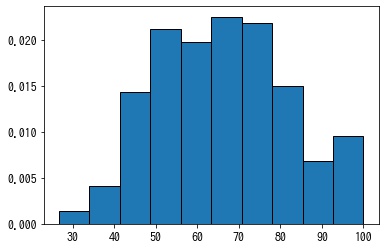

1.0000000000000002

累積ヒストグラムを作成する

cumulative=True とした場合、累積ヒストグラムになります。

In [6]:

np.random.seed(0)

x = np.random.normal(65, 15, 200).clip(0, 100)

fig, ax = plt.subplots()
ax.hist(x, cumulative=True, ec="k")

plt.show()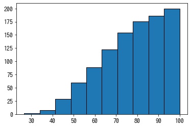

cumulative=-1 とした場合、右から左へ累積させる累積ヒストグラムになります。

In [7]:

np.random.seed(0)

x = np.random.normal(65, 15, 200).clip(0, 100)

fig, ax = plt.subplots()
ax.hist(x, cumulative=-1, ec="k")

plt.show()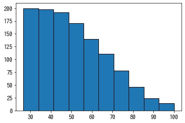

ヒストグラムの描画方法を設定する

histtype でヒストグラムの描画方法を指定できます。

histtype="bar": 棒でヒストグラムを描画します。
histtype="step": ヒストグラムの外形を線で描画します。
histtype="stepfilled": ヒストグラムの外形を塗りつぶして描画します。

In [8]:

np.random.seed(0)

x = np.random.normal(65, 15, 200).clip(0, 100)

fig, axes = plt.subplots(1, 3, figsize=(9, 3))

for p, ax in zip(["bar", "step", "stepfilled"], axes):
    ax.hist(x, histtype=p, ec="k")
    ax.set_title(f'histtype="{p}"')

plt.show()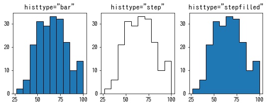

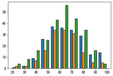
複数のデータのヒストグラムを作成する場合に、histtype="barstacked" を指定した場合、異なるデータの棒を並べて表示する代わりに積み上げて表示します。

In [9]:

np.random.seed(0)

x1 = np.random.normal(65, 15, 200).clip(0, 100)
x2 = np.random.normal(65, 15, 150).clip(0, 100)
X = [x1, x2]

fig, axes = plt.subplots(1, 2, figsize=(9, 3))

for p, ax in zip(["bar", "barstacked"], axes):
    ax.hist(X, histtype=p, ec="k")
    ax.set_title(f'histtype="{p}"')

plt.show()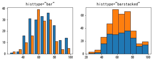

ヒストグラムの位置を指定する。

align でヒストグラムの棒の x 方向の配置を指定できます。

"left": 棒の中央をビンに左端に来るように配置します。
"mid": 棒の中央をビンに中央に来るように配置します。
"right": 棒の中央をビンに右端に来るように配置します。

In [10]:

np.random.seed(0)

x = np.random.normal(65, 20, 200).clip(0, 100)

fig, axes = plt.subplots(3, 1, figsize=(5, 8))

for p, ax in zip(["left", "mid", "right"], axes):
    ax.hist(x, bins=np.linspace(0, 100, 11), align=p, ec="k", rwidth=0.5)
    ax.set_title(f'align="{p}"')
    ax.set_xticks(np.linspace(0, 100, 11))

fig.tight_layout()
plt.show()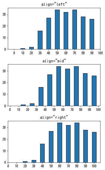

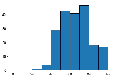
ヒストグラムの向きを設定する

orientation="horizontal" を指定した場合、横向きのヒストグラムになります。

In [11]:

np.random.seed(0)

x = np.random.normal(65, 15, 200).clip(0, 100)

fig, ax = plt.subplots()
ax.hist(x, orientation="horizontal", ec="k")

plt.show()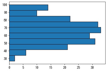

棒の幅を設定する

rwidth を指定した場合、棒の幅をビンの幅の割合で指定できます。デフォルトは 1 なので、棒は隙間なく並べられます。

In [12]:

np.random.seed(0)

x = np.random.normal(65, 15, 200).clip(0, 100)

fig, ax = plt.subplots()
ax.hist(x, rwidth=0.5, ec="k")

plt.show()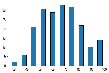

棒の色を設定する

color で棒の色を指定できます。

In [13]:

np.random.seed(0)

x = np.random.normal(65, 15, 200).clip(0, 100)

fig, ax = plt.subplots()
ax.hist(x, color="g", ec="k")

plt.show()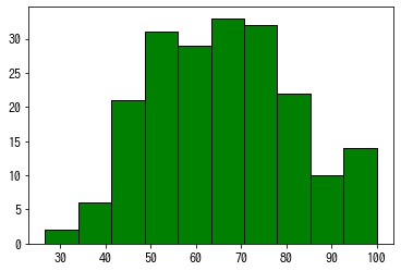

複数のデータのヒストグラムを作成する場合は、color に色の一覧を指定します。

In [14]:

np.random.seed(0)

x1 = np.random.normal(65, 15, 200).clip(0, 100)
x2 = np.random.normal(65, 15, 150).clip(0, 100)
x3 = np.random.normal(65, 15, 250).clip(0, 100)
X = [x1, x2, x3]

fig, ax = plt.subplots()
ax.hist(X, label=["x1", "x2", "x3"], color=["r", "g", "b"], ec="k")
ax.legend()

plt.show()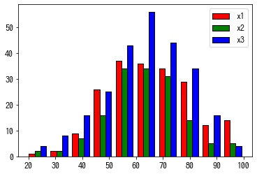

pyplot.hist() の返り値

各ビンの度数、ビンの端、描画オブジェクトの3つの返り値を返します。

In [15]:

np.random.seed(0)

x = np.random.normal(65, 15, 200).clip(0, 100)

fig, ax = plt.subplots()
n, bins, patches = ax.hist(x, ec="k")
print(n)
print(bins)
print(patches)

plt.show()

[ 2.  6. 21. 31. 29. 33. 32. 22. 10. 14.]
[ 26.70515276  34.03463749  41.36412221  48.69360693  56.02309166
  63.35257638  70.6820611   78.01154583  85.34103055  92.67051528
 100.        ]
<a list of 10 Patch objects>

In [16]:

np.random.seed(0)

x1 = np.random.normal(65, 15, 200).clip(0, 100)
x2 = np.random.normal(65, 15, 150).clip(0, 100)
x3 = np.random.normal(65, 15, 250).clip(0, 100)
X = [x1, x2, x3]

fig, ax = plt.subplots()
n, bins, hist = ax.hist(X, ec="k")
print(n)
print(bins)
print(patches)

plt.show()

[[ 1.  2.  9. 26. 37. 36. 34. 29. 12. 14.]
 [ 2.  2.  7. 16. 34. 34. 31. 14.  5.  5.]
 [ 4.  8. 16. 25. 43. 56. 44. 34. 16.  4.]]
[ 19.30785418  27.37706876  35.44628334  43.51549792  51.58471251
  59.65392709  67.72314167  75.79235625  83.86157084  91.93078542
 100.        ]
<a list of 10 Patch objects>