
概要
matplotlib の pyplot.hist2d() で2次元ヒストグラムを作成する方法について解説します。
pyplot.hist2d
matplotlib.pyplot.hist2d(x, y, bins=10, range=None, density=False, weights=None, cmin=None, cmax=None, *, data=None, **kwargs)| 名前 | 型 | デフォルト値 |
|---|---|---|
| x, y | array-like, shape (n, ) | |
| 入力値。 | ||
| bins | None or int or [int, int] or array-like or [array, array] | 10 |
| ビン | ||
| range | array-like shape(2, 2) | None |
| 各次元ごとのビンの左端と右端を [[xmin, xmax], [ymin, ymax]] の形式で指定します。この範囲外の値はすべて外れ値とみなされ、集計されません。 | ||
| density | bool, default: False | False |
| True の場合、ヒストグラムを確率密度になるように正規化します。 | ||
| weights | array-like, shape (n, ) | None |
| An array of values w_i weighing each sample (x_i, y_i). | ||
| cmin, cmax | float, default: None | |
| 度数が cmin より小さいか cmax より大きいすべてのビンは表示されず、返り値の度数も NaN になります。 | ||
| 名前 | 説明 |
|---|---|
| 2D array | 2次元ヒストグラムの度数 |
| 1D array | x 軸のビンの端。 |
| 1D array | y 軸のビンの端。 |
| QuadMesh | ヒストグラムを表すオブジェクト |
2次元ヒストグラム
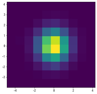
2次元ヒストグラムとは、2次元のデータを、2次元をグリッド上に分割して作成したビンを元に作成するヒストグラムです。
import numpy as np
from matplotlib import pyplot as plt
from numpy.random import multivariate_normal

np.random.seed(0)

# データを作成する。
x, y = np.random.multivariate_normal([0, 0], [[1, 0], [0, 1]], size=100000).T
print(x.shape, y.shape)  # (100000,) (100000,)

fig, ax = plt.subplots(figsize=(6, 6))
ax.hist2d(x, y)

plt.show()
(100000,) (100000,)
ビンの指定方法
整数で指定した場合、x 方向、y 方向を共に bins 等分してビンを作成します。
np.random.seed(0)

x, y = np.random.multivariate_normal([0, 0], [[1, 0], [0, 1]], size=100000).T

fig, ax = plt.subplots(figsize=(6, 6))
h, xedges, yedges, img = ax.hist2d(x, y, bins=10)

ax.set_xticks(xedges)
ax.set_yticks(yedges)
ax.grid()

plt.show()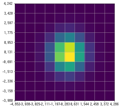
bins=[xbins, ybins] と指定した場合、x 方向を xbins 等分、y 方向を ybins 等分して、ビンを作成します。
np.random.seed(0)

x, y = np.random.multivariate_normal([0, 0], [[1, 0], [0, 1]], size=100000).T

fig, ax = plt.subplots(figsize=(6, 6))
h, xedges, yedges, img = ax.hist2d(x, y, bins=[8, 10])

ax.set_xticks(xedges)
ax.set_yticks(yedges)
ax.grid()

plt.show()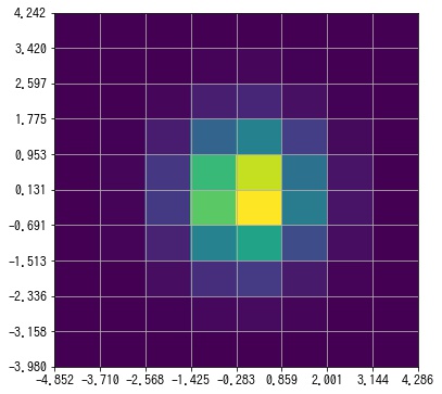
bins=[v0, v1, ..., vn] と指定した場合、x 方向、y 方向のビンの端が共に [v0, v1, ..., vn] となるようにビンを作成します。
np.random.seed(0)

x, y = np.random.multivariate_normal([0, 0], [[1, 0], [0, 1]], size=100000).T

fig, ax = plt.subplots(figsize=(6, 6))
h, xedges, yedges, img = ax.hist2d(x, y, bins=np.linspace(-5, 5, 11))

ax.set_xticks(xedges)
ax.set_yticks(yedges)
ax.grid()

plt.show()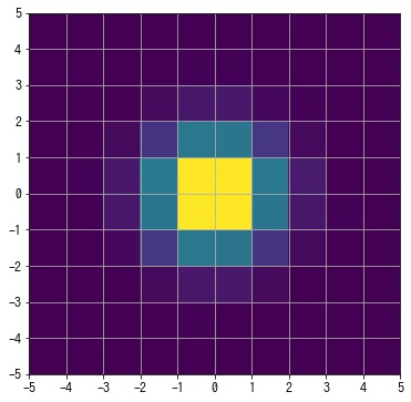
bins=[[x0, x1, ..., xn], [y0, y1, ..., yn]] と指定した場合、x 方向のビンの端が [v0, v1, ..., vn]、y 方法のビンの端が [y0, y1, ..., yn] となるようにビンを作成します。
np.random.seed(0)

x, y = np.random.multivariate_normal([0, 0], [[1, 0], [0, 1]], size=100000).T

fig, ax = plt.subplots(figsize=(6, 6))
h, xedges, yedges, img = ax.hist2d(
    x, y, bins=[np.linspace(-5, 5, 11), np.linspace(-8, 8, 17)]
)

# bins を描画する。
ax.set_xticks(xedges)
ax.set_yticks(yedges)
ax.grid()

plt.show()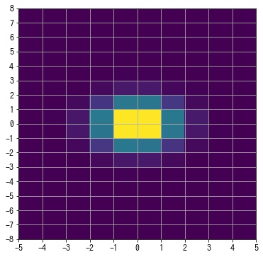
ビンを作成する範囲を設定する
デフォルトでは全データが収まる範囲 range=[[xmin, xmax], [ymin, ymax]] でビンが作成されますが、range で集計対象の範囲を指定できます。
np.random.seed(0)

x, y = np.random.multivariate_normal([0, 0], [[1, 0], [0, 1]], size=100000).T

fig, ax = plt.subplots(figsize=(6, 6))
h, xedges, yedges, img = ax.hist2d(x, y, range=[[-2, 2], [-2, 2]])

# bins を描画する。
ax.set_xticks(xedges)
ax.set_yticks(yedges)
ax.grid()

plt.show()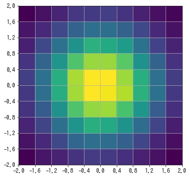
ヒストグラムを正規化する
normed=True を指定すると、確率密度関数になるように正規化します。つまり、各ビンの面積にそのビンの度数を乗算した総和が1になります。
ビンの度数の総和が1になるように正規化されるわけではないことに注意してください。ビンの度数の総和が1になるように正規化したい場合は、weights 引数で各サンプルの重みを 1 / 全データ数 としてヒストグラムを計算します。
np.random.seed(0)

x, y = np.random.multivariate_normal([0, 0], [[1, 0], [0, 1]], size=100000).T

fig, ax = plt.subplots(figsize=(6, 6))
h, xedges, yedges, img = ax.hist2d(x, y, bins=10, density=True)

# ヒストグラムを確率密度関数と解釈して、積分した値が1となるように正規化する。
ws = xedges[1:] - xedges[:-1]
hs = yedges[1:] - yedges[:-1]
print(np.sum(ws * hs * h))  # 1.0

# ヒストグラムの総和を1にしたい場合は weights で調整する。
h, xedges, yedges, img = ax.hist2d(x, y, bins=10, weights=np.ones_like(x) / len(x))
print(h.sum())  # 1.000000000000015
0.9999999999999999 1.000000000000014
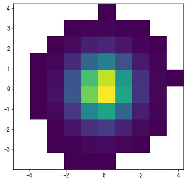
頻度値が指定した範囲外のビンは非表示にする。
cmin, cmax を指定した場合、度数が cmin 未満及び cmax より大きいビンは非表示になり、返り値の度数の値も NaN になります。
np.random.seed(0)

x, y = np.random.multivariate_normal([0, 0], [[1, 0], [0, 1]], size=100000).T

fig, ax = plt.subplots(figsize=(6, 6))
h, xedges, yedges, img = ax.hist2d(x, y, bins=10, cmin=10)

print(h)

plt.show()
[[ nan nan nan nan nan nan nan nan nan nan] [ nan nan nan 28. 27. 49. 21. nan nan nan] [ nan 22. 76. 292. 475. 424. 218. 40. nan nan] [ 11. 80. 565. 1693. 2923. 2800. 1300. 329. 32. nan] [ 23. 230. 1480. 4972. 8425. 7563. 3568. 939. 120. nan] [ 27. 325. 1886. 6266. 10724. 9766. 4655. 1158. 169. 13.] [ nan 198. 1053. 3501. 6318. 5669. 2692. 648. 92. nan] [ nan 36. 290. 919. 1625. 1552. 754. 146. 21. nan] [ nan nan 40. 119. 194. 183. 101. 23. nan nan] [ nan nan nan nan nan 13. nan nan nan nan]]
カラーマップを設定する
cmap でカラーマップを指定できます。指定可能なカラーマップは以下の記事を参照してください。
[blogcard url=”https://pystyle.info/matplotlib-colormap”]
np.random.seed(0)

x, y = np.random.multivariate_normal([0, 0], [[1, 0], [0, 1]], size=100000).T

fig, ax = plt.subplots(figsize=(6, 6))
h, xedges, yedges, img = ax.hist2d(x, y, cmap="magma")

plt.show()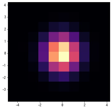
コメント