機械学習 – ベイズの識別規則

1. 概要
2. 損失行列
3. 損失関数
4. ベイズ識別規則 (Bayes’ decision rule)
5. 最大事後確率識別識別とベイズの識別識別の関係
6. 例: 2クラス分類

概要

ベイズの識別規則について解説します。以下の記事の続きになります。

機械学習 – 決定理論ついて (ML 識別規則、MAP 識別規則) – pystyle

損失行列

$(i, j)$ 成分を正解のクラスが $c_i$ の入力 $\bm{x}$ を $c_j$ と分類した場合の損失とした行列を損失行列 (loss matrix) といい、$L$ で表します。

損失関数

入力 $\bm{x}$ をクラス $c_i$ と分類した場合の損失を損失関数 (loss function) またはコスト関数 (cost function) で定義します。

$$ r(c_i|\bm{x}) = \sum_{j = 1}^K L_{ij} p(c_j|\bm{x}) $$

ベイズ識別規則 (Bayes’ decision rule)

損失関数 $r(c_i|\bm{x})$ が最小となるクラスに割り当てる識別規則をベイズ識別規則 (Bayes’ decision rule) といいます。

識別関数

$$ g_i(\bm{x}) = -r(c_i|\bm{x}), (i = 1, 2, \cdots, K) $$

決定境界

クラス $c_i$ の決定領域は

$$ \mathcal{R}_i = \{\bm{x} \in \R^d| c_i = \argmin_j r(c_j|\bm{x})\} $$

識別クラス

入力 $\bm{x}$ の識別クラス $\hat{y}$ は

$$ \begin{aligned} \hat{y} &= \argmin_i r(c_i|\bm{x}) \\ &= c_i \ \text{s.t.} \ r(c_i|\bm{x}) \le r(c_j|\bm{x}), (i \ne j) \end{aligned} $$

期待損失

ベイズ識別規則の期待損失を

$$ \varepsilon = E[\min_i r(c_i|\bm{x})] $$

と定義すると、

$$ \begin{aligned} \varepsilon &= E[\min_j r(c_j|\bm{x})] \\ &= \int_{\R^d} \min_j r(c_j|\bm{x}) p(\bm{x}) d\bm{x} \quad \because 期待値の定義 \\ &= \sum_{i = 1}^K \int_{\mathcal{R}_i} \min_j r(c_j|\bm{x}) p(\bm{x}) d\bm{x} \quad \because \mathcal{R}_1, \mathcal{R}_2, \cdots, \mathcal{R}_K は \R^d の分割 \\ &= \sum_{i = 1}^K \int_{\mathcal{R}_i} r(c_i|\bm{x}) p(\bm{x}) d\bm{x} \quad \because \bm{x} \in \mathcal{R}_i \to r(c_i|\bm{x}) = \min_j r(c_j|\bm{x}) \\ &= \sum_{i = 1}^K \sum_{j = 1}^K \int_{\mathcal{R}_i} L_{ij} p(c_j|\bm{x}) p(\bm{x}) d\bm{x} \quad \because r(c_i|\bm{x}) の定義 \\ &= \sum_{i = 1}^K \sum_{j = 1}^K \int_{\mathcal{R}_i} L_{ij} p(\bm{x}|c_j) p(c_j) d\bm{x} \quad \because ベイズの定理 \\ \end{aligned} $$

最大事後確率識別識別とベイズの識別識別の関係

損失行列を $L_{ii} = 0, L_{ij} = 1, (i \ne j)$ とすると、

$$ L = \begin{pmatrix} 0 & 1 & \cdots 1 \\ 1 & 0 & \cdots 1 \\ \vdots & \vdots & \cdots \vdots \\ 1 & 1 & \cdots 0 \\ \end{pmatrix} $$

これを zero-one loss といいます。

このとき、ベイズの識別規則は最大事後確率識別識別と一致します。

$$ \begin{aligned} \hat{y} &= \argmin_i r(c_i|\bm{x}) \\ &= \argmin_i \sum_{j = 1}^K L_{ij} p(c_j|\bm{x}) \\ &= \argmin_i \sum_{i \ne j} p(c_j|\bm{x}) \quad \because L_{ii} = 0, L_{ij} = 1 \\ &= \argmin_i 1 – p(c_i|\bm{x}) \quad \because \sum_{i = 1}^K p(c_i|\bm{x}) = 1 \\ &= \argmax_i p(c_i|\bm{x}) \end{aligned} $$

例: 2クラス分類

釣った魚の大きさが $x \in \R$ であったとき、その魚が鮭 (salmon)、スズキ (sea bass) のどちらであるかを識別する2クラス分類問題を考えます。(鮭、スズキ以外の魚が釣れることはないと仮定します)

以下の情報がわかっているものとします。

事前確率
- 釣った魚が鮭である確率は $p(salmon) = \frac{2}{3}$
- 釣った魚がスズキである確率は $p(bass) = \frac{1}{3}$
尤度
- 鮭の大きさは正規分布 $\mathcal{N}(5, 1)$ に従う $$ p(x|salmon) = \frac{1}{\sqrt{2 \pi}} \exp \left( -\frac{(x – 5)^2}{2} \right) $$
- スズキの大きさは正規分布 $\mathcal{N}(10, 4)$ に従う $$ p(x|bass) = \frac{1}{2 \sqrt{2 \pi}} \exp \left( -\frac{(x – 10)^2}{8} \right) $$
損失行列

鮭はスズキより高価でおいしいため、鮭をスズキと間違って分類した場合は損失が大きくなるものとして、次のように損失を定義します。

鮭をスズキと間違って識別した場合は2
スズキを鮭と間違って識別した場合は1
正解した場合は0

このとき、損失行列は次のようになります。

$$ L = \begin{pmatrix} 0 & 3 \\ 1 & 0 \end{pmatrix} $$

損失は

$$ \begin{aligned} r(salmon|x) &= L_{11} p(salmon|\bm{x}) + L_{12} p(bass|\bm{x}) \\ &= L_{11} p(\bm{x}|salmon)p(salmon) + L_{12} p(\bm{x}|bass)p(bass) \\ &= 3 \times \frac{1}{2 \sqrt{2 \pi}} \exp \left( -\frac{(x – 10)^2}{8} \right) \times \frac{1}{3} \end{aligned} $$$$ \begin{aligned} r(bass|x) &= L_{21} p(salmon|\bm{x}) + L_{22} p(bass|\bm{x}) \\ &= L_{21} p(\bm{x}|salmon)p(salmon) + L_{22} p(\bm{x}|bass)p(bass) \\ &= 1 \times \frac{1}{\sqrt{2 \pi}} \exp \left( -\frac{(x – 5)^2}{2} \right) \times \frac{2}{3} \end{aligned} $$

このとき、ベイズ識別規則に従うと、予測クラスは

$$ \begin{aligned} \hat{y} &= \begin{cases} salmon & \text{if} \ r(salmon|x) \le r(bass|x) \\ bass & \text{if} \ r(salmon|x) > r(bass|x) \end{cases} \\ \end{aligned} $$

$r(salmon|x), r(bass|x)$ を描画すると以下のようになります。

In [1]:

import matplotlib.pyplot as plt
import numpy as np
from scipy.stats import norm

x = np.linspace(0, 20, 100)

salmon_y = norm.pdf(x, loc=10, scale=2)
bass_y = norm.pdf(x, loc=5, scale=1) * 2 / 3

fig, ax = plt.subplots(figsize=(9, 6))
ax.plot(x, salmon_y, "b", label=r"$r(salmon|x)$")
ax.plot(x, bass_y, "g", label=r"$r(bass|x)$")

ax.set_xlabel("Length")
ax.grid()
ax.legend()

plt.show()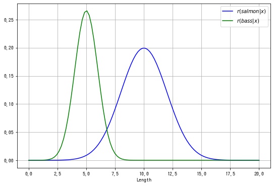

このとき、鮭とスズキの決定領域は以下になります。

$$ \begin{aligned} \mathcal{R}_{salmon} &= \{\bm{x} \in \R^d| r(salmon|x) \le r(bass|x) \} \\ \mathcal{R}_{bass} &= \{\bm{x} \in \R^d| r(salmon|x) > r(bass|x) \} \end{aligned} $$

Sympy で $r(salmon|x) = r(bass|x)$ を解いて、最尤識別規則の決定境界を計算します

In [2]:

import sympy as sym
from sympy.stats import density, Normal

x = sym.symbols("x")

salmon_r = density(Normal("bass", 10, 2))(x)
bass_r = density(Normal("salmon", 5, 1))(x) * 2 / 3

# 方程式を解く。
ret = sym.solve(salmon_r - bass_r)

# 数値解にする。
x1, x2 = sym.N(ret[0]), sym.N(ret[1])
print(x1, x2)

-0.113152312119997 6.77981897878666

前の記事

機械学習 – 決定理論について 2020.07.09
次の記事

機械学習 – 最尤識別規則 2020.07.10