
目次
概要
データをクラスに分類する識別規則について解説します。
識別規則
入力に対して、それを1つのクラスに割り当てる規則を識別規則 (decision rule) といいます。
判別関数
クラス $c_1, c_2, \cdots, c_K$ の $K$ クラス分類問題を考えます。 識別規則は、識別関数 (discriminant function) $g_i: \R^d \to \R, (i = 1, 2, \cdots, K)$ によって定義されます。 入力 $\bm{x} \in \R^d$ が与えられたとき、判別関数 $g_i(\bm{x})$ の値が最大となるクラス $\hat{y}$ を割り当てます。
$$ \begin{aligned} \hat{y} &= \argmax_i g_i(\bm{x}) \\ &= c_i \ \text{s.t.} \ g_i(\bm{x}) \ge g_j(\bm{x}), (i \ne j) \end{aligned} $$決定領域
入力 $\bm{x}$ が与えられたときそれがクラス $c_i$ と識別される領域を、クラス $c_i$ の決定領域 (decision region) といいます。
クラス $c_i$ の決定領域 $\mathcal{R}_i$ は
$$ \mathcal{R}_i = \{\bm{x} \in \R^d| c_i = \argmax_j g_j(\bm{x})\} $$決定領域は、入力データの定義域を分割します。
$$ \begin{aligned} \R^d &= \bigcup_{i = 1}^K \mathcal{R}_i \\ \mathcal{R}_i \cap \mathcal{R}_j &= \varnothing, (i, j = 1, 2, \cdots, K, i \ne j) \end{aligned} $$決定領域同士の境界を決定境界 (decision boundary) といいます。
例: scikit-learn で決定領域を描画する
scikit-learn で2次元の3クラスのデータセットをロジスティクス回帰モデルで学習し、決定領域を可視化します。
In [1]:
import matplotlib.pyplot as plt
import numpy as np
from matplotlib.colors import ListedColormap
from sklearn import datasets
from sklearn.datasets import make_blobs
from sklearn.linear_model import LogisticRegression

# データを作成する。
X, y = make_blobs(
    random_state=0, n_samples=200, n_features=2, cluster_std=0.8, centers=3
)

# ロジスティック回帰モデルで学習する。
model = LogisticRegression(solver="lbfgs", multi_class="multinomial")
model.fit(X, y)

fig, ax = plt.subplots(figsize=(8, 6))

# 入力値を描画する。
ax.scatter(X[y == 0, 0], X[y == 0, 1], c="r", s=10, label="Class $c_1$")
ax.scatter(X[y == 1, 0], X[y == 1, 1], c="b", s=10, label="Class $c_2$")
ax.scatter(X[y == 2, 0], X[y == 2, 1], c="g", s=10, label="Class $c_3$")

# 決定領域を描画する。
XX, YY = np.meshgrid(
    np.linspace(*ax.get_xlim(), 1000), np.linspace(*ax.get_ylim(), 1000)
)
XY = np.column_stack([XX.ravel(), YY.ravel()])
ZZ = model.predict(XY).reshape(XX.shape)
ax.contourf(XX, YY, ZZ, alpha=0.2, cmap=ListedColormap(["r", "b", "g"]))

ax.legend()

plt.show()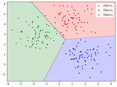
- 赤の決定領域のデータはクラス $c_1$ と識別される
- 青の決定領域のデータはクラス $c_2$ と識別される
- 緑の決定領域のデータはクラス $c_3$ と識別される
- 決定領域同士の境目は決定境界
コメント